Lecture Notes: ConvNets using Torch
We will be using Torch for this lab. We already know how to implement a linear layer and softmax layer. We will be re-using some code from the previous lab for Sections 1, and 2. In this lecture we will be exclusively using Torch, so the forward (prediction) and backward (gradient computation) functions are already implemented.
1. First let's load some training data.
We will be using the CIFAR-10 dataset. CIFAR-10 is a dataset consisting of 50k training images belonging to 10 categories. A validation set is also provided which contains 10k images. We have a version of this dataset here that has all the images resized to 32x32. This is a relatively small dataset so it is very convenient to experiment with. You will probably read several papers reporting results on this dataset during this class but most state-of-the-art methods usually try experiments in much larger datasets with millions of images.
require 'image'
-- The default tensor type in Torch is DoubleTensor, but we generally only need Float precision.
torch.setdefaulttensortype('torch.FloatTensor')

-- Load data.
trainset = torch.load('cifar10-train.t7') -- training images.
valset = torch.load('cifar10-val.t7')  -- validation set used to evaluate the model and tune parameters.
trainset.label = trainset.label + 1
valset.label = valset.label + 1
classes = {'airplane', 'automobile', 'bird', 'cat', 'deer',
           'dog', 'frog', 'horse', 'ship', 'truck'}

-- Let's show all images of frogs.
class2ids = {}  -- Build a mapping between object names and class ids.
-- Remember that tables in lua are similar to (key,value) collections e.g. hashmaps.
for k,v in pairs(classes) do class2ids[v] = k end

-- Retrieve the frog class number.
object_class_id = class2ids['frog'] -- try changing this to visualize some images from other categories.
-- Put all images of frogs into a table.
objects = {}
local object_indices = trainset.label:eq(object_class_id):nonzero():squeeze()
for i = 1, 36 do  -- Let's show the first 36 frogs.
    table.insert(objects, trainset.data[object_indices[i]])
end

-- Plot the images of frogs using itorch.image
itorch.image(objects)
print(trainset) -- View what is inside the training set.
print(valset)  -- View what is inside the validation set.

2. Preprocessing and normalizing the data.
The images in this dataset are already pre-processed a bit, they are all 3x32x32, this means they have three channels (RGB), and they all have a width and height of 32 pixels. It is also generally a good idea in machine learning to center the inputs around zero. Each RGB value in our ByteTensor inputs goes from 0 to 255. We want the values to go from -1 to 1, if possible. This sometimes makes learning a function on these inputs easier.
-- Make the data a FloatTensor.
trainset.normdata = trainset.data:clone():float()
valset.normdata = valset.data:clone():float()
cifarMean = {trainset.normdata[{{}, {1}, {}, {}}]:mean(),
             trainset.normdata[{{}, {2}, {}, {}}]:mean(),
             trainset.normdata[{{}, {3}, {}, {}}]:mean()}

cifarStd = {trainset.normdata[{{}, {1}, {}, {}}]:std(),
            trainset.normdata[{{}, {2}, {}, {}}]:std(),
            trainset.normdata[{{}, {3}, {}, {}}]:std()}

-- Print the mean and std value for each channel.
print(cifarMean)
print(cifarStd)

-- Now normalize the training and validation data.
for i  = 1, 3 do
    -- Subtracting the mean on each channel makes the values roughly between -128 and 128.
    trainset.normdata[{{}, {i}, {}, {}}]:add(-cifarMean[i])
    valset.normdata[{{}, {i}, {}, {}}]:add(-cifarMean[i])
    -- Dividing the std on each channel makes the values roughly between -1 and 1.
    trainset.normdata[{{}, {i}, {}, {}}]:div(cifarStd[i])
    valset.normdata[{{}, {i}, {}, {}}]:div(cifarStd[i])
end
3. Torch code for Linear Softmax + SGD from the last lecture
Here is the code that builds a linear model and runs mini-batch SGD to learn the parameters of the model. We will modify in this lab the model to 1) Use multiple two linear layers and a non-linear activation function. and 2) Use two convolutional layers and two linear layers. Additionally, I introduced some changes in the training loop to support a custom provided feature tensor, and a preprocessing function for later sections in this Lab.
require 'nn'  -- This library contains the classes we will need (Linear, LogSoftMax, ClassNLLCriterion)

local model = nn.Sequential()   -- Just a container of sequential operations.
model:add(nn.View(32 * 32 * 3))  -- This View layer vectorizes the images from a 3,32,32 tensor to a 3*32*32 vector.
model:add(nn.Linear(32 * 32 * 3, 10))  -- Linear transformation y = Wx + b
model:add(nn.LogSoftMax())  -- Log SoftMax function.

local criterion = nn.ClassNLLCriterion() -- Negative log-likelihood criterion.
-- params is a flat vector with the concatenation of all the parameters inside model.
-- gradParams is a flat vector with the concatenation of all the gradients of parameters inside the model.
-- These two variables also merely point to the internal individual parameters in each layer of the module.

function trainModel(model, opt, features, preprocessFn)
    -- Get all the parameters (and gradients) of the model in a single vector.
    local params, gradParams = model:getParameters()

    local opt = opt or {}
    local batchSize = opt.batchSize or 64  -- The bigger the batch size the most accurate the gradients.
    local learningRate = opt.learningRate or 0.001  -- This is the learning rate parameter often referred to as lambda.
    local momentumRate = opt.momentumRate or 0.9
    local numEpochs = opt.numEpochs or 3
    local velocityParams = torch.zeros(gradParams:size())
    local train_features, val_features
    if preprocessFn then
        train_features = trainset.data:float():div(255)
        val_features = valset.data:float():div(255)
    else
        train_features = (features and features.train_features) or trainset.normdata
        val_features = (features and features.val_features) or valset.normdata
    end
    -- Go over the training data this number of times.
    for epoch = 1, numEpochs do
        local sum_loss = 0
        local correct = 0

        -- Run over the training set samples.
        model:training()
        for i = 1, trainset.normdata:size(1) / batchSize do

            -- 1. Sample a batch.
            local inputs
            if preprocessFn then
                inputs = torch.Tensor(batchSize, 3, 224, 224)
            else
                inputs = (features and torch.Tensor(batchSize, 4096)) or torch.Tensor(batchSize, 3, 32, 32)
            end
            local labels = torch.Tensor(batchSize)
            for bi = 1, batchSize do
                local rand_id = torch.random(1, train_features:size(1))
                if preprocessFn then
                    inputs[bi] = preprocessFn(train_features[rand_id])
                else
                    inputs[bi] = train_features[rand_id]
                end
                labels[bi] = trainset.label[rand_id]
            end
            -- 2. Perform the forward pass (prediction mode).
            local predictions = model:forward(inputs)

            -- 3. Evaluate results.
            for i = 1, predictions:size(1) do
                local _, predicted_label = predictions[i]:max(1)
                if predicted_label[1] == labels[i] then correct = correct + 1 end
            end
            sum_loss = sum_loss + criterion:forward(predictions, labels)

            -- 4. Perform the backward pass (compute derivatives).
            -- This zeroes-out all the parameters inside the model pointed by variable params.
            model:zeroGradParameters()
            -- This internally computes the gradients with respect to the parameters pointed by gradParams.
            local gradPredictions = criterion:backward(predictions, labels)
            model:backward(inputs, gradPredictions)

            -- 5. Perform the SGD update.
            velocityParams:mul(momentumRate)
            velocityParams:add(learningRate, gradParams)
            params:add(-1, velocityParams)

            if i % 100 == 0 then  -- Print this every five thousand iterations.
                print(('train epoch=%d, iteration=%d, avg-loss=%.6f, avg-accuracy = %.2f')
                    :format(epoch, i, sum_loss / i, correct / (i * batchSize)))
            end
        end

        -- Run over the validation set for evaluation.
        local validation_accuracy = 0
        local nBatches = val_features:size(1) / batchSize
        model:evaluate()
        for i = 1, nBatches do

            -- 1. Sample a batch.
            if preprocessFn then
                inputs = torch.Tensor(batchSize, 3, 224, 224)
            else
                inputs = (features and torch.Tensor(batchSize, 4096)) or torch.Tensor(batchSize, 3, 32, 32)
            end
            local labels = torch.Tensor(batchSize)
            for bi = 1, batchSize do
                local rand_id = torch.random(1, val_features:size(1))
                if preprocessFn then
                    inputs[bi] = preprocessFn(val_features[rand_id])
                else
                    inputs[bi] = val_features[rand_id]
                end
                labels[bi] = valset.label[rand_id]
            end

            -- 2. Perform the forward pass (prediction mode).
            local predictions = model:forward(inputs)

            -- 3. evaluate results.
            for i = 1, predictions:size(1) do
                local _, predicted_label = predictions[i]:max(1)
                if predicted_label[1] == labels[i] then validation_accuracy = validation_accuracy + 1 end
            end
        end
        validation_accuracy = validation_accuracy / (nBatches * batchSize)
        print(('\nvalidation accuracy at epoch = %d is %.4f'):format(epoch, validation_accuracy))
    end
end

trainModel(model)
4. Torch code for a 2-layer Neural Network.
We only need to modify the code for the model and add another linear layer and an activation function in-between.
local model = nn.Sequential()   -- Just a container of sequential operations.
model:add(nn.View(32 * 32 * 3))  -- This View layer vectorizes the images from a 3,32,32 tensor to a 3*32*32 vector.
model:add(nn.Linear(32 * 32 * 3, 500))  -- Linear transformation y = Wx + b
model:add(nn.ReLU())
model:add(nn.Linear(500, 10))  -- Linear transformation y = Wx + b
model:add(nn.LogSoftMax())  -- Log SoftMax function.

trainModel(model) -- Reuse our training code from earlier.
Using the code above you probably experience a significant improvement in performance. Does adding more layers will keep improving perforamnce?
5. Torch code for a Convolutional Neural Network.
We pass the input image through two convolutional layers and then apply two linear layers. This model does not vectorize the input images right away. It first passes the images through two layers of convolutional filtering, then vectorizes this output and passes it to a neural network with two linear layers.
local model = nn.Sequential()
model:add(nn.SpatialConvolution(3, 8, 5, 5))  -- 3 input channels, 8 output channels (8 filters), 5x5 kernels.
model:add(nn.ReLU())
model:add(nn.SpatialMaxPooling(2, 2, 2, 2)) -- Max pooling in 2 x 2 area.
model:add(nn.SpatialConvolution(8, 16, 5, 5))  -- 8 input channels, 16 output channels (16 filters), 5x5 kernels.
model:add(nn.ReLU())
model:add(nn.SpatialMaxPooling(2, 2, 2, 2))  -- Max pooling in 2 x 2 area.
model:add(nn.View(16*5*5))   -- Vectorize the output of the convolutional layers.
model:add(nn.Linear(16*5*5, 120))
model:add(nn.ReLU())
model:add(nn.Linear(120, 84))
model:add(nn.ReLU())
model:add(nn.Linear(84, 10))
model:add(nn.LogSoftMax())

opt = {}
opt.learningRate = 0.01 -- bigger learning rate worked best for this network.
opt.batchSize = 32  -- smaller batch size, less accurate gradients, but more frequent updates.
opt.numEpochs = 5
trainModel(model, opt)
6. Torch code for a Convolutional Neural Network with BatchNorm.
We pass the input image through two convolutional layers and then apply two linear layers. A good idea that has become recently popular is BatchNormalization which consists in a layer that normalizes the output of the previous layer in a similar way that we normalized the input in Section 2. Here is how to incorporate that.
local model = nn.Sequential()
model:add(nn.SpatialConvolution(3, 8, 5, 5))  -- 3 input channels, 8 output channels (8 filters), 5x5 kernels.
model:add(nn.SpatialBatchNormalization(8, 1e-3))  -- BATCH NORMALIZATION LAYER.
model:add(nn.ReLU())
model:add(nn.SpatialMaxPooling(2, 2, 2, 2)) -- Max pooling in 2 x 2 area.
model:add(nn.SpatialConvolution(8, 16, 5, 5))  -- 8 input channels, 16 output channels (16 filters), 5x5 kernels.
model:add(nn.SpatialBatchNormalization(16, 1e-3))  -- BATCH NORMALIZATION LAYER.
model:add(nn.ReLU())
model:add(nn.SpatialMaxPooling(2, 2, 2, 2))  -- Max pooling in 2 x 2 area.
model:add(nn.View(16*5*5))    -- Vectorize the output of the convolutional layers.
model:add(nn.Linear(16*5*5, 120))
model:add(nn.ReLU())
model:add(nn.Linear(120, 84))
model:add(nn.ReLU())
model:add(nn.Linear(84, 10))
model:add(nn.LogSoftMax())

opt = {}
opt.learningRate = 0.02 -- bigger learning rate worked best for this network.
opt.batchSize = 32  -- smaller batch size, less accurate gradients, but more frequent updates.
opt.numEpochs = 5
trainModel(model, opt)  -- This will take a while!
7. Running a pre-trained Imagenet Model on your Images
As you start realizing from the last experiment, it can take very long to train one of these models (and require much more memory), especially if you have many convolutional layers with hundreds of filters. The state-of-the-art models contain up to 150 layers (here we used 4) and are trained with at least 1 million images (here we used 50k) to predict 1000 categories (here we used 10). Training these models requires days or weeks of training using a GPU or an array of them. GPUs can accelerate the operations of these models up to 70x compared to using CPUs.
In our experiment below we will execute a variant of the AlexNet model, which was the architecture proposed in:
by Alex Krizhevsky, Ilya Sutskever, and Geoff Hinton.
require 'nn' -- just in case not loaded earlier.

-- Load the class list.
imagenetClasses = torch.load('alexnetowtbn_classes.t7')   -- This is the list of 1000 classes of Imagenet ILSVRC.
meanStd = torch.load('alexnetowtbn_meanStd.t7')  -- This is the mean and std used for normalizing images.

-- Load the model.
model = torch.load('alexnetowtbn_epoch55_cpu.t7')
model:evaluate()  -- Turn on evaluate mode. This is important for layers like BatchNorm or Dropout!
-- print(model)  -- This shows detailed information about every layer in the model.
Here I'm showing using an image the relevant parts of how this model is composed. The convolutional layers in charge of feature extraction are grouped under a Sequential container, and the classification layers are grouped in a second Sequential container: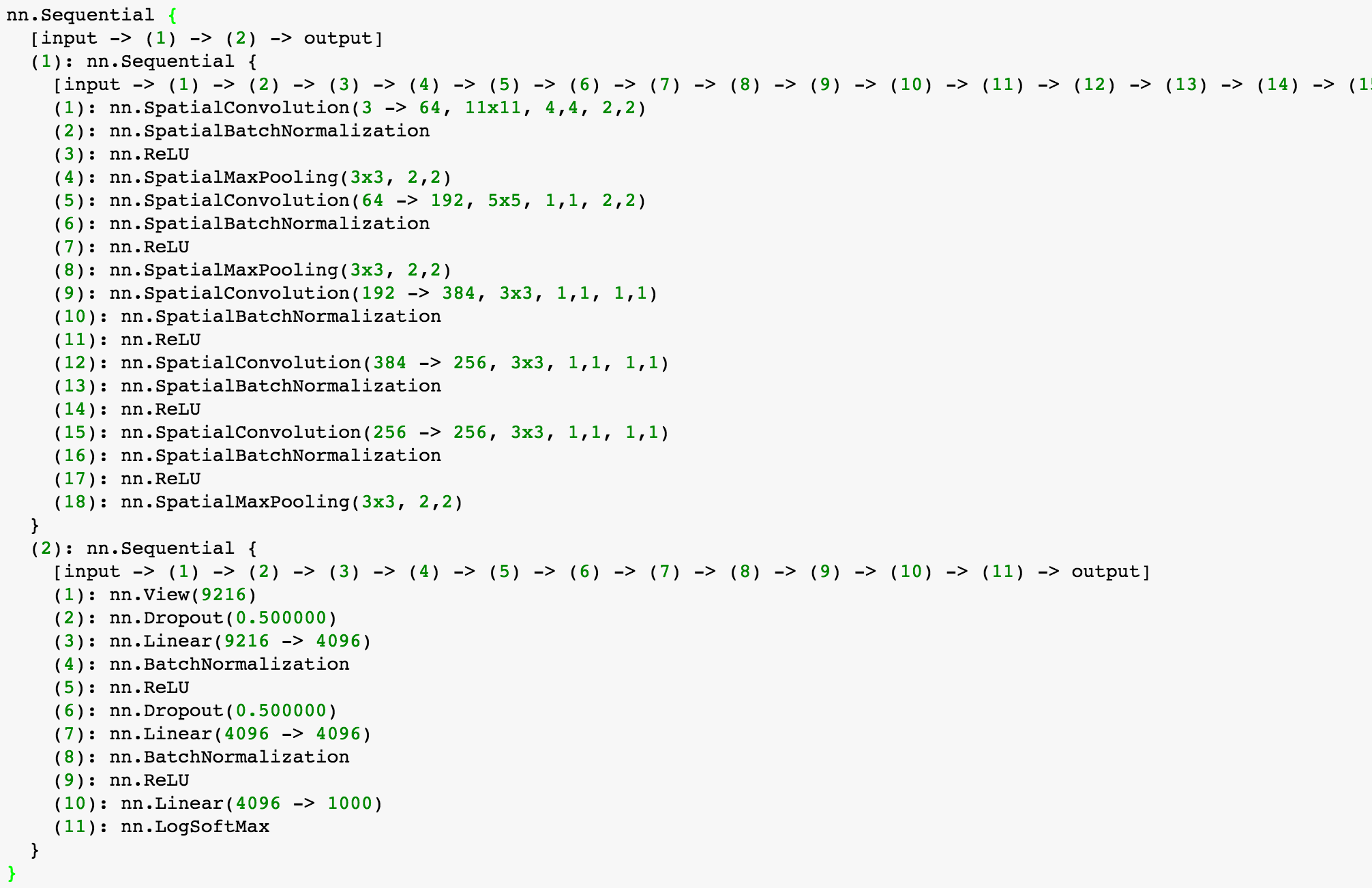
Now that we have our model loaded let's run an image through it and examine its predictions. Note that this model was trained using images resized to 256x256 and taking a center crop of size 224x224. We can up-size images from CIFAR-10 and run them through the network. Let's try that with an image of a frog or a bird.
local input_image = image.load('bird.jpg', 3, 'float') -- make it a float and between 0 and 1.
input_image = image.scale(input_image, 224, 224)  -- resize to the appropriate input for this network.
itorch.image(input_image)

-- Pre-process the image channel by channel.
function preprocess(im)
    local output_image = image.scale(im:clone(), 224, 224)
    for i = 1, 3 do -- channels
        output_image[{{i},{},{}}]:add(-meanStd.mean[i])
        output_image[{{i},{},{}}]:div(meanStd.std[i])
    end
    return output_image
end

input_image = preprocess(input_image):view(1, 3, 224, 224) -- put it in batch form by adding another dimension.

local predictions = model:forward(input_image)
-- Remember that the last layer is a LogSoftMax so we need to exp() that.
local scores, classIds = predictions[1]:exp():sort(true)

for i = 1, 5 do
    print(('[%s] = %.5f'):format(imagenetClasses[classIds[i]], scores[i]))
end
8. Transfer learning I: Intermediate Network Outputs as Features
A powerful idea is using the pre-trained network on Imagenet and repurpose it for other tasks. A simple way to do this is using the activations of the network from the layer before the last linear layer as image features. Let's try to do this for the CIFAR task that we were training earlier. First, let's compute the activations for the last convolutional layer for all images to use these as features (just like we used the vectorized image representation, or color histograms). The following code will probably take a while (about 30 minutes). If you have a GPU this code will be blazing fast. There are a few modifications you will have to make to the code so it runs in the GPU (e.g. model:cuda(), batchTensor:cuda(), and maybe model = cudnn.convert(model, cudnn) to add cudnn support)
function compute_features(input_images)
    -- Create a tensor to hold the feature vectors.
    local features = torch.FloatTensor(input_images:size(1), 4096):zero()
    local batch_size = 250   -- Let's process images in groups of 128.
    for i = 1, input_images:size(1) / batch_size do
        local batchTensor = torch.FloatTensor(batch_size, 3, 224, 224)
        for j = 1, batch_size do
            local im = input_images[(i - 1) * batch_size + j]
            batchTensor[j] = preprocess(im)
        end
        -- Pass the pre-processed images through the network but discard the predictions.
        model:forward(batchTensor)
        -- Store the intermediate results from the layer before the prediction layer.
        for j = 1, batch_size do
            features[(i - 1) * batch_size + j] = model:get(2):get(9).output[j]
        end
        print(('%d. Features computed for %d out of %d images'):format(i, i * batch_size, input_images:size(1)))
    end
    return features
end

local train_images = trainset.data:float():div(255)
local val_images = valset.data:float():div(255)
features = {}
features.train_features = compute_features(train_images)
features.val_features = compute_features(val_images)
torch.save('alexnet_features.t7', features)  -- just in case this notebook gets closed.
Now let's just try a 2-layer neural network using the computed features.
-- features = torch.load('alexnet_features.t7') -- in case these are not already in memory.

local model = nn.Sequential()   -- Just a container of sequential operations.
model:add(nn.Linear(4096, 500))  -- Linear transformation y = Wx + b
model:add(nn.ReLU())
model:add(nn.Linear(500, 10))  -- Linear transformation y = Wx + b
model:add(nn.LogSoftMax())  -- Log SoftMax function.

opt = {}
opt.learningRate = 0.01
opt.numEpochs = 5
trainModel(model, opt, features) -- Reuse our training code from earlier.
9. Transfer learning II: Fine-tuning the Network
An even stronger tool for transfer learning is modifying and adapting the AlexNet network parameters directly using SGD for a different task. This process is often referred to as fine-tuning the network. Here I show code to perform that for CIFAR, this requires forward and backward propagation on this pre-trained network and it will be a slow process (unless you use a GPU for this part).
-- Make sure the AlexNet model is loaded.
require 'nn' -- Make sure nn is loaded.
model = torch.load('alexnetowtbn_epoch55_cpu.t7')

-- Remove the last Linear layer of the model which is meant to predict 1000 classes.
model:get(2):remove(11) -- Remove the LogSoftMax layer.
model:get(2):remove(10) -- Remove the last Linear layer (4096 -> 1000)

-- Replace this last layer with a new Linear layer meant to predict 10 classes.
model:add(nn.Linear(4096, 10))  -- Add back a Linear layer (4096 -> 10)
model:add(nn.LogSoftMax())  -- Add back the LogSoftMax layer.

opt = {}
opt.learningRate = 0.001
opt.numEpochs = 5
opt.batchSize = 16
trainModel(model, opt, {}, preprocess) -- Reuse our training code from earlier.
Lab Questions
- Include a table here reporting the loss and final accuracy for each model in Sections 4, 5, 6, and 8 (no need to run section 9 unless you have a GPU where you can easily run it).
- Visualize the convolutional filters for the first convolutional layer of the model in section 5 before and after training. Do so by rescaling the values appropriately to show them as RGB images. (Check the Torch documentation to find how to retrieve them from the model variable)
- Similarly visualize the convolutional filters corresponding to the first convolutional layer of the pre-trained AlexNet model of section 7.
- The AlexNet model that was used in this lab occupies 466MB. Include a table here detailing how much of this space is occupied layer by layer.
- Why does the AlexNet model presented in this lab must have a nn.View layer with an input dimension of 9216?
- More powerful models were proposed after AlexNet, one of them is known as the VGG model (see code here https://github.com/soumith/imagenet-multiGPU.torch/blob/master/models/vggbn.lua), another one is the GoogLenet model (see code here https://github.com/soumith/imagenet-multiGPU.torch/blob/master/models/googlenet.lua). Describe here in one paragraph each, what are the architectural differences and innovations that you notice with respect to the AlexNet model (e.g. more layers? how many more? more filters? bigger convolutional filters? smaller convolutional filters? Just by looking at the code can you estimate which model occupies more memory VGG or GoogLenet?).