Deep Learning Lab
If you are taking this class you have some experience with machine learning. You probably already have used or at the very least have heard about deep learning. There are many deep learning libraries that allow you to easily create neural networks. For Python, the following are some libraries that I recommend based on my own experience or good experiences from other people I trust: PyTorch, Keras (using Theano or Tensorflow), MXNet, Chainer, Lasagne. These libraries are all nice, and we will use them for our later labs and maybe the class project, but in this lab will be creating our own deep learning library: PyDeepTensorNet!
1. Single-layer neural network
First, let's review the skeleton of a single linear layer neural network. The inputs of the network are the variables $x_1, x_2, x_3, x_4$, or the input vector $x=[x_1, x_2, x_3, x_4]$, the outputs of the network are $a_1,a_2,a_3$, or the output vector $a=[a_1,a_2,a_3]$:
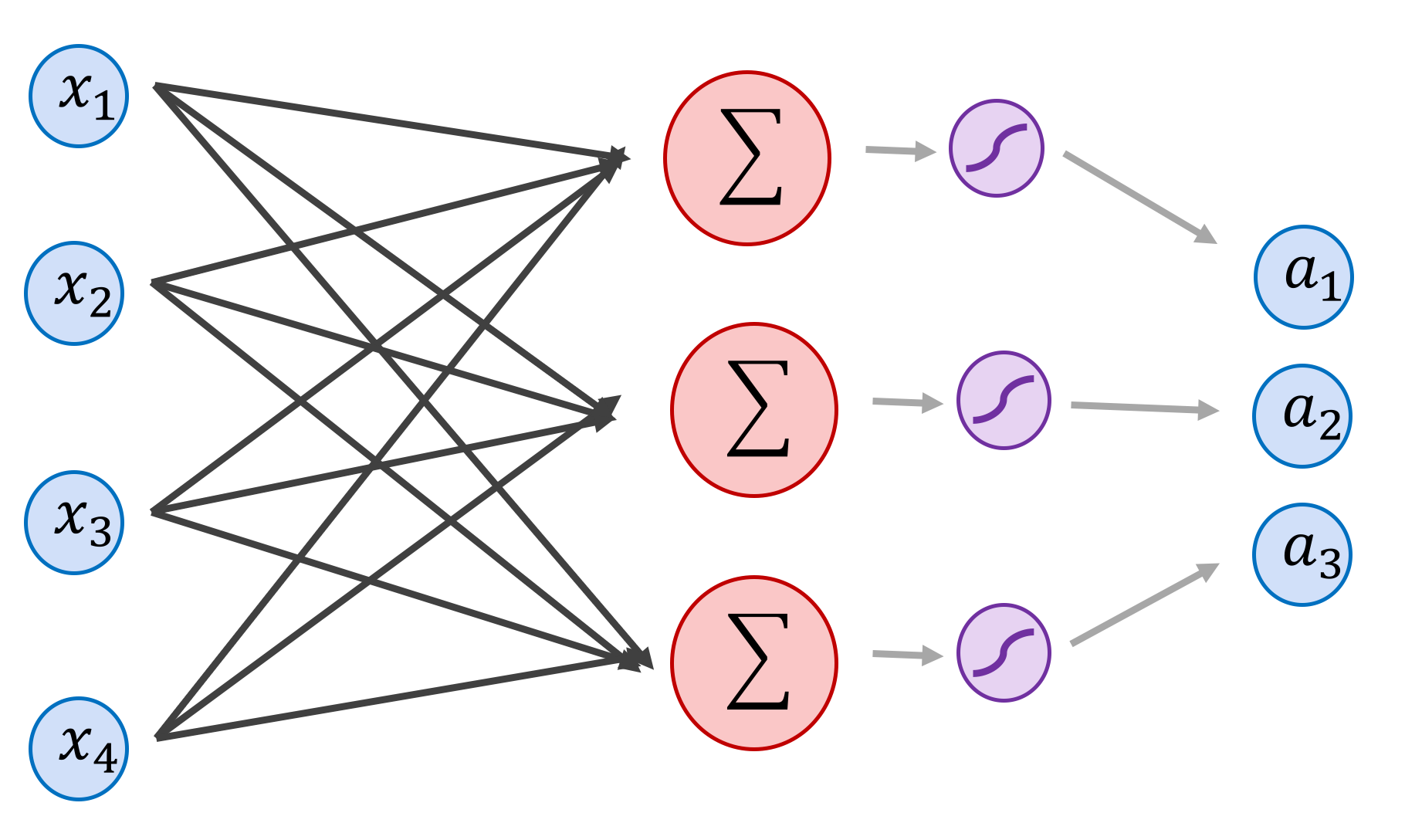
The outputs $a_i$ of this single linear layer + activation function are computed as follows:
$$a_j= \text{sigmoid}(w_{1j}x_1 + w_{2j}x_2 + w_{3j}x_3 + w_{4j}x_4 + b_j) = \text{sigmoid}\Big(\sum_{i=1}^{i=4}w_{ij}x_{i} + b_j\Big)$$In matrix notation, this would be: (note the intentional capitalization of the word sigmoid, which now operates element-wise)
\begin{equation} \begin{bmatrix} a_{1} \\ a_{2} \\ a_{3} \end{bmatrix}^T=\text{Sigmoid}\Bigg( \begin{bmatrix} x_{1} \\ x_{2} \\ x_{3} \\ x_{4} \end{bmatrix}^T \begin{bmatrix} w_{1,1} & w_{1,2} & w_{1,3}\\ w_{2,1} & w_{3,2} & w_{2,3}\\ w_{3,1} & w_{3,2} & w_{3,3}\\ w_{4,1} & w_{4,2} & w_{4,3} \end{bmatrix} + \begin{bmatrix} b_{1} \\ b_{2} \\ b_{3} \end{bmatrix}^T\Bigg) \end{equation}The sigmoid function is: $sigmoid(x) = 1 \;/\; (1 + exp(-x))$, or alternatively: $sigmoid(x) = exp(x)\;/\;(1 + exp(x))$, however in practice this can be (and often is) replaced by other functions that we will discuss later. We will separate the sigmoid logically into an activation layer $\sigma(x)$ and a linear layer $\text{linear}(3,4)$
These two rather simple operations are at the core of all neural networks. A lot of work goes into finding the right set of weights in the matrix $W$ and bias vector $b$ so that the outputs $a$ predict something useful based on the inputs $x$. Training these weights $W$ requires having many training pairs $(a^{(m)}, x^{(m)})$ for your task. The inputs $x$ can be the pixels of an image, indices of words, the entries in a database, and the outputs $a$ can also be literally anything, including a number indicating a category, a set of numbers indicating the indices of words composing a sentence, an output image itself, etc.
2. Forward-propagation
When we compute the outputs $a$ from the inputs $x$ in this network composed of a single linear layer, and a sigmoid layer, this process is called forward-propagation. Let's implement these two operations below:
import numpy as np
import numpy.matlib

class nn_Sigmoid:
    def forward(self, x):
        return 1 / (1 + np.exp(-x))

class nn_Linear:
    def __init__(self, input_dim, output_dim):
        # Initialized with random numbers from a gaussian N(0, 0.001)
        self.weight = np.matlib.randn(input_dim, output_dim) * 0.001
        self.bias = np.matlib.randn((1, output_dim)) * 0.001

    # y = Wx + b
    def forward(self, x):
        return np.dot(x, self.weight) + self.bias

    def getParameters(self):
        return [self.weight, self.bias]

# Let's test the composition of the two functions (forward-propagation in the neural network).
x1 = np.array([[1, 2, 2, 3]])
a1 = nn_Sigmoid().forward(nn_Linear(4, 3).forward(x1))
print('x[1] = '+ str(x1))
print('a[1] = ' + str(a1))

# Let's test the composition of the two functions (forward-propagation in the neural network).
x2 = np.array([[4, 5, 2, 1]])
a2 = nn_Sigmoid().forward(nn_Linear(4, 3).forward(x2))
print('x[2] = '+ str(x2))
print('a[2] = ' + str(a2))

# We can also compute both at once, which could be more efficient since it requires a single matrix multiplication.
x = np.concatenate((x1, x2), axis = 0)
a = nn_Sigmoid().forward(nn_Linear(4, 3).forward(x))
print('x = ' + str(x))
print('a = ' + str(a))
3. Loss functions.
After computing the output predictions $a$ it is necessary to compare these against the true values of $a$. Let's call these true, correct, or desired values $y$. A simple loss or cost function is used to measure the degree by which the prediction $a$ is wrong with respect to $y$. A common loss function for regression is the sum of squared differences between the prediction and its true value. Assuming a prediction $a^{(d)}$ for our training sample $x^{(d)}$ with true value $y^{(d)}$, then the loss can be computed as:
$$loss(a^{(d)}, y^{(d)}) = (a^{(d)}_1 - y^{(d)}_1)^2 + (a^{(d)}_2 - y^{(d)}_2)^2 + (a^{(d)}_3 - y^{(d)}_3)^2 = \sum_{j=1}^{j=3}(a^{(d)}_j - y^{(d)}_j)^2$$We want to modify the parameters [weight, bias] in our Linear layer so that the value of $loss(a^{(d)}, y^{(d)})$ becomes as small as possible for all training samples in a set $D=\{(x^{(d)},y^{(d)})\}$ so that our predictions $a$ are as similar as possible to the true values $y$. So the function we are really trying to minimize is the following:
$$Loss(W, b) = \sum_{d=1}^{d=|D|} loss(a^{(d)}, y^{(d)})$$The only two variables for our model in the function $Loss$ are $W$ and $b$, this is because the training dataset $D$ is fixed. We need to find how to move the values of $W$ and $b$ so that $Loss$ is minimal. In order to calculate the minimum of this function we can compute the derivatives of the function and find the zeroes:
$$\frac{\partial Loss}{\partial w_{i,j}} \quad\text{ and }\quad \frac{\partial Loss}{\partial b_{j}} $$This can be easily accomplished for some models, for instance if we did not have the the $\text{sigmoid}$ function, this problem would be standard linear regression and we could find a formula that would give us the parameters right away. You can check in wikipedia a derivation of the normal equations for linear least squares here. However, we will take a different approach and solve this problem by iteratively following the direction of an approximate gradient using Stochastic Gradient Descent (SGD) because this will be used for more complex models. We will also compute the derivatives using the Backpropagation algorithm.
class nn_MSECriterion:  # MSE = mean squared error.
    def forward(self, predictions, labels):
        return np.sum(np.square(predictions - labels))

# Let's test the loss function.
y_hat = np.array([[0.23, 0.25, 0.33], [0.23, 0.25, 0.33], [0.23, 0.25, 0.33], [0.23, 0.25, 0.33]])
y_true = np.array([[0.25, 0.25, 0.25], [0.33, 0.33, 0.33], [0.77, 0.77, 0.77], [0.80, 0.80, 0.80]])
print nn_MSECriterion().forward(y_hat, y_true)
4. Backward-propagation (Backpropagation)
Backpropagation is just applying the chain-rule in calculus to compute the derivative of a function which is the composition of many functions (which is essentially what neural networks are all about). To start, let's make one important observation: that $Loss(W, b)$ (uppercase) is a sum of $loss$ functions (lowercase) for each sample in the dataset, and therefore its derivative can be computed as the sum of the derivatives of $loss$ (the loss for each sample $(x^{(d)},y^{(d)})$).
So we wil concentrate on finding the derivative of the following function with respect to each parameter:
$$loss(W,b) = f(g(h(W,b))$$where $f$, $g$, and $h$ are the least squares loss, the sigmoid function, and a linear transformation respectively:
\begin{align} f(u) &= (u - y^{(d)})^2 && \text{Remember here that }y^{(d)}\text{ is a constant, and } u=g(v)\\ g(v) &= \frac{1}{1 - e^{-v}} && \text{where } v = h(W, b)\\ h(W,b) &= \Big[\sum_{i=1}^{i=4}w_{ij}x^{(d)}_{i} + b_j\Big] && \text{Remember here that }x^{(d)}\text{ is a constant and } h(W,b) \text{ outputs a vector with $j$ entries.} \end{align}So we can compute the partial derivative $\frac{\partial loss(W,b)}{\partial w_{i,j}}$ by using the chain rule as follows:
$$\frac{\partial loss(W,b)}{\partial w_{i,j}} = \frac{\partial f(u)}{\partial u} \frac{\partial g(v)}{\partial v} \frac{\partial h(W,b)}{\partial w_{i,j}}$$The derivatives for each of these functions are: (please verify the derivations on your own)
\begin{align} \frac{\partial f(u)}{\partial u} &= 2(u - y^{(d)})\\\\ \frac{\partial g(v)}{\partial v} &= g(v)(1 - g(v))\\\\ \frac{\partial h(W,b)}{\partial w_{ij}} = x^{(d)}_{i} &\quad\text{ and }\quad \frac{\partial h(W,b)}{\partial b_{j}} = 1\quad\text{ and }\quad \frac{\partial h(W,b)}{\partial x_{i}} = \sum_{j=1}^{j=3}w^{(d)}_{ij} \end{align}Here we will implement these derivative computations:
# This is referred above as f(u).
class nn_MSECriterion:
    def forward(self, predictions, labels):
        return np.sum(np.square(predictions - labels))

    def backward(self, predictions, labels):
        num_samples = labels.shape[0]
        return num_samples * 2 * (predictions - labels)

# This is referred above as g(v).
class nn_Sigmoid:
    def forward(self, x):
        return 1 / (1 + np.exp(-x))

    def backward(self, x, gradOutput):
        # It is usually a good idea to use gv from the forward pass and not recompute it again here.
        gv = 1 / (1 + np.exp(-x))
        return np.multiply(np.multiply(gv, (1 - gv)), gradOutput)

# This is referred above as h(W, b)
class nn_Linear:
    def __init__(self, input_dim, output_dim):
        # Initialized with random numbers from a gaussian N(0, 0.001)
        self.weight = np.matlib.randn(input_dim, output_dim) * 0.01
        self.bias = np.matlib.randn((1, output_dim)) * 0.01
        self.gradWeight = np.zeros_like(self.weight)
        self.gradBias = np.zeros_like(self.bias)

    def forward(self, x):
        return np.dot(x, self.weight) + self.bias

    def backward(self, x, gradOutput):
        # dL/dw = dh/dw * dL/dv
        self.gradWeight = np.dot(x.T, gradOutput)
        # dL/db = dh/db * dL/dv
        self.gradBias = np.copy(gradOutput)
        # return dL/dx = dh/dx * dL/dv
        return np.dot(gradOutput, self.weight.T)

    def getParameters(self):
        params = [self.weight, self.bias]
        gradParams = [self.gradWeight, self.gradBias]
        return params, gradParams


# Let's test some dummy inputs for a full pass of forward and backward propagation.
x1 = np.array([[1, 2, 2, 3]])
y1 = np.array([[0.25, 0.25, 0.25]])

# Define the operations.
linear = nn_Linear(4, 3)  # h(W, b)
sigmoid = nn_Sigmoid()  # g(v)
loss = nn_MSECriterion()  # f(u)

# Forward-propagation.
a0 = linear.forward(x1)
a1 = sigmoid.forward(a0)
loss_val = loss.forward(a1, y1) # Loss function.

# Backward-propagation.
da1 = loss.backward(a1, y1)
da0 = sigmoid.backward(a0, da1)
dx1 = linear.backward(x1, da0)

# Show parameters of the linear layer.
print('\nW = ' + str(linear.weight))
print('B = ' + str(linear.bias))

# Show the intermediate outputs in the forward pass.
print('\nx1 = '+ str(x1))
print('a0 = ' + str(a0))
print('a1 = ' + str(a1))

print('\nloss = ' + str(loss_val))

# Show the intermediate gradients with respect to inputs in the backward pass.
print('\nda1 = ' + str(da1))
print('da0 = ' + str(da0))
print('dx1 = ' + str(dx1))

# Show the gradients with respect to parameters.
print('\ndW = ' + str(linear.gradWeight))
print('dB = ' + str(linear.gradBias))
5. Gradient Checking
The gradients can also be computed with numerical approximation using the definition of derivatives. Let a single input pair $(x, y)$ be the input, for each entry $w_{ij}$ in the weight matrix $W$ we are interested in the following:
$$\frac{\partial loss(W,b)}{\partial w_{ij}} = \frac{loss(W + \mathcal{E}_{ij},b) - loss(W - \mathcal{E}_{ij}, b)}{2\epsilon}, $$where $\mathcal{E}_{ij}$ is a matrix that has $\epsilon$ in its $(i,j)$ entry and zeros everywhere else. Intuitively this gradient tells us how would the value of the loss changes if we shake a particular weight $w_{ij}$ by an $\epsilon$ amount. We can do the same to compute derivatives with respect to the bias parameters $b_i$. Here is a piece of code that checks for a given input $(x, y)$, the gradients for the matrix $W$.
# We will compute derivatives with respect to a single data pair (x,y)
x = np.array([[2.34, 3.8, 34.44, 5.33]])
y = np.array([[3.2, 4.2, 5.3]])

# Define the operations.
linear = nn_Linear(4, 3)
sigmoid = nn_Sigmoid()
criterion = nn_MSECriterion()

# Forward-propagation.
a0 = linear.forward(x)
a1 = sigmoid.forward(a0)
loss = criterion.forward(a1, y) # Loss function.

# Backward-propagation.
da1 = criterion.backward(a1, y)
da0 = sigmoid.backward(a0, da1)
dx = linear.backward(x, da0)

gradWeight = linear.gradWeight
gradBias = linear.gradBias

approxGradWeight = np.zeros_like(linear.weight)
approxGradBias = np.zeros_like(linear.bias)

# We will verify here that gradWeights are correct and leave it as an excercise
# to verify the gradBias.
epsilon = 0.0001
for i in range(0, linear.weight.shape[0]):
    for j in range(0, linear.weight.shape[1]):
        # Compute f(w)
        fw = criterion.forward(sigmoid.forward(linear.forward(x)), y) # Loss function.
        # Compute f(w + eps)
        shifted_weight = np.copy(linear.weight)
        shifted_weight[i, j] = shifted_weight[i, j] + epsilon
        shifted_linear = nn_Linear(4, 3)
        shifted_linear.bias = linear.bias
        shifted_linear.weight = shifted_weight
        fw_epsilon = criterion.forward(sigmoid.forward(shifted_linear.forward(x)), y) # Loss function
        # Compute (f(w + eps) - f(w)) / eps
        approxGradWeight[i, j] = (fw_epsilon - fw) / epsilon

# These two outputs should be similar up to some precision.
print('gradWeight: ' + str(gradWeight))
print('\napproxGradWeight: ' + str(approxGradWeight))
6. Stochastic Gradient Descent.
We are almost ready to train our model. We will use a dummy dataset that we will generate automatically below. The inputs are 1000 vectors of size 4, and the outputs are 1000 vectors of size 3. We will just focus on training, however keep in mind that in a real task we would be interested in the accuracy of the model on test (unseen) data.
dataset_size = 1000

# Generate random inputs within some range.
x = np.random.uniform(0, 6, (dataset_size, 4))
# Generate outputs based on the inputs using some function.
y1 = np.sin(x.sum(axis = 1))
y2 = np.sin(x[:, 1] * 6)
y3 = np.sin(x[:, 1] + x[:, 3])
y = np.array([y1, y2, y3]).T

print(x.shape)
print(y.shape)
Now that we compute gradients efficiently we will implement the stochastic gradient descent loop that moves the weights according to the gradients. In each iteration we sample an (input, label) pair and compute the gradients of the parameters, then we update the parameters according to the following rules:
$$w_{ij} = w_{ij} - \lambda\frac{\partial \ell}{\partial w_{ij}}$$$$b_i = b_i - \lambda\frac{\partial \ell}{\partial b_i}$$where $\lambda$ is the learning rate.
learningRate = 0.1

model = {}
model['linear'] = nn_Linear(4, 3)
model['sigmoid'] = nn_Sigmoid()
model['loss'] = nn_MSECriterion()

for epoch in range(0, 400):
    loss = 0
    for i in range(0, dataset_size):
        xi = x[i:i+1, :]
        yi = y[i:i+1, :]

        # Forward.
        a0 = model['linear'].forward(xi)
        a1 = model['sigmoid'].forward(a0)
        loss += model['loss'].forward(a1, yi)

        # Backward.
        da1 = model['loss'].backward(a1, yi)
        da0 = model['sigmoid'].backward(a0, da1)
        model['linear'].backward(xi, da0)

        model['linear'].weight = model['linear'].weight - learningRate * model['linear'].gradWeight
        model['linear'].bias = model['linear'].bias - learningRate * model['linear'].gradBias

    if epoch % 10 == 0: print('epoch[%d] = %.8f' % (epoch, loss / dataset_size))
Lab Questions (5 pts) [Include your code and intermediate outputs]
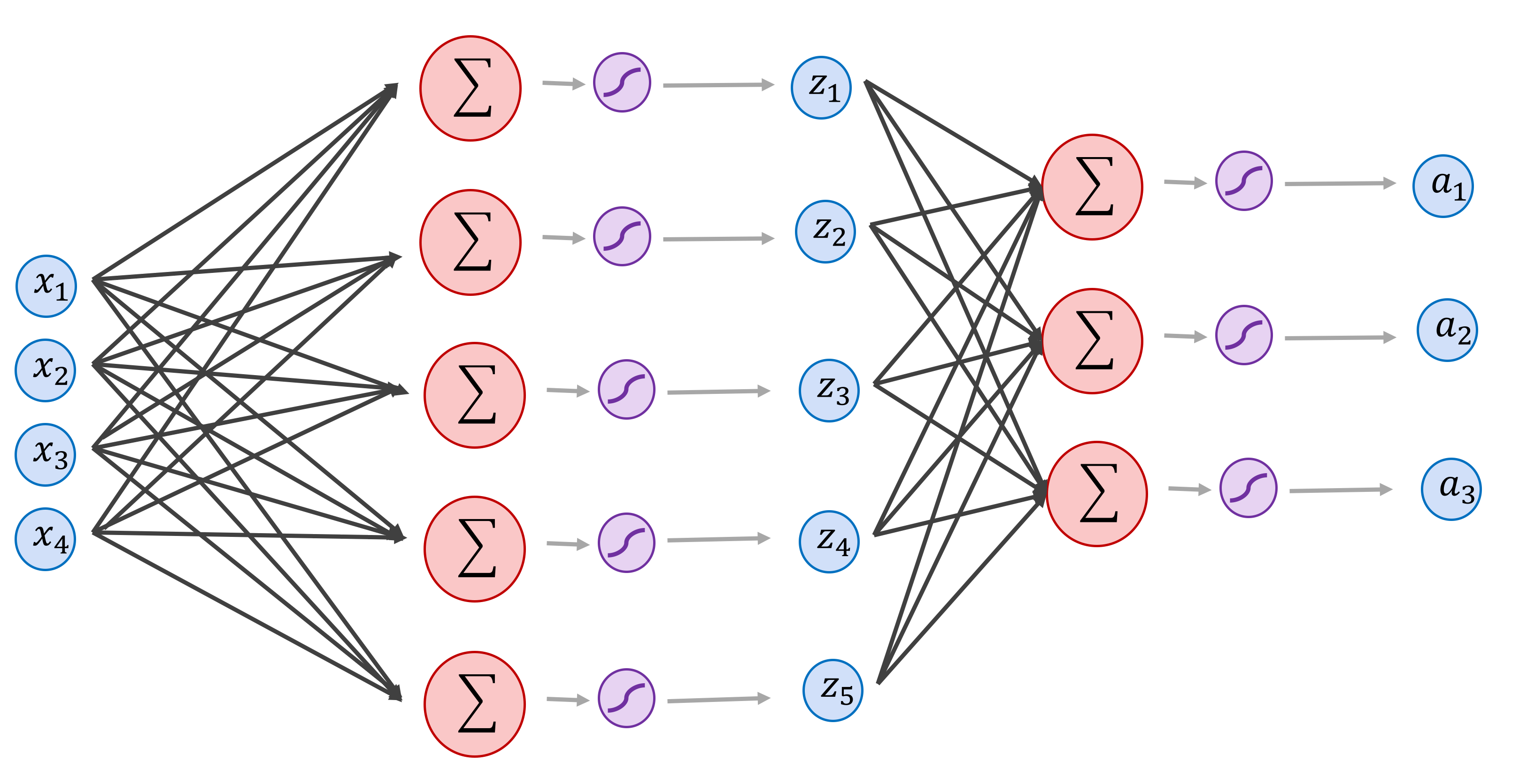
1) In Section 6. We implemented a single layer neural network that takes as input vectors of size 4, and outputs vectors of size 3. Modify the code from section 6 to train the network below (use the same dummy dataset and print the final loss using the same number of epochs) [2pts]:
# Your code goes here.
2) Check the gradients of the above network for both linear layer parameters $W_1$ and $W_2$ using some sample input x, and y. (You can look at the code from section 5 for this) [1pt]
# Your code goes here.
3) There are other activation functions that can be used instead of sigmoid. Implement below the forward and backward operation for the following functions [1pt]:
$$\text{ReLU}(x) = \text{max}(0, x)$$Note, that the above $\text{max}$ operates element-wise on the input vector $x$.
$$\text{Tanh(x)} = \text{tanh}(x) = \frac{e^{x} - e^{-x}}{e^{x} + e^{-x}}$$# Rectified linear unit
class nn_ReLU:
def forward(self, x):
# Forward pass.
def backward(self, x, gradOutput):
# Backward pass
# Hyperbolic tangent.
class nn_Tanh:
def forward(self, x):
# Forward pass.
def backward(self, x, gradOutput):
# Backward pass
4) There are other loss functions that can be used instead of a mean squared error criterion. Implement the forward and backward operations for the following loss functions where $a$ is a vector of predicted values, and $y$ is the vector with ground-truth labels (both vectors are of size $n$) [1pts]:
$$\text{AbsCriterion}(y, a) = \frac{1}{n}\sum_{i=1}^{i=n}|y_i - a_i|$$$$\text{BinaryCrossEntropy}(y, a) = \frac{1}{n}\sum_{i=1}^{i=n} [y_i\text{log}(a_i) + (1 - y_i)\text{log}(1 - a_i)]$$,
The binary cross entropy loss assumes that the vector $y$ only has values that are either 0 and 1, and the prediction vector $a$ contains values between 0 and 1 (e.g. the output of a $\text{sigmoid}$ layer).
# Absolute difference criterion or L-1 distance criterion.
class nn_AbsCriterion:
    def forward(self, predictions, labels):
        # Forward pass.

    def backward(self, predictions, labels):
        # Backward pass.

# Binary cross entropy criterion. Useful for classification as opposed to regression.
class nn_BCECriterion:
    def forward(self, predictions, labels):
        # Forward pass.

    def backward(self, predictions, labels):
        # Backward pass.
Optional: Most deep learning libraries support batches, meaning you can forward, and backward a set of inputs. Our library PyDeepTensorNet supports batches in the forward pass (review again section 2 where we input two vectors to the network). However, our backward pass does not support batches. Modify the code in backward function of the nn_Linear class to support batches. Then test your implementation by training the network in section 6 using a batch size of 32 [2pts]. (Keep in mind that the gradWeight and gradBias vectors should accumulate the gradients of each input in the batch. This is because the gradient of the loss with respect to the batch is the sum of the gradients with respect to each sample in the batch).