Backward algorithm

Like the forward algorithm, we can use the backward algorithm to calculate the marginal likelihood of a hidden Markov model (HMM). Also like the forward algorithm, the backward algorithm is an instance of dynamic programming where the intermediate values are probabilities.

Recall the forward matrix values can be specified as:

f_k,i = P(x_1..i,π_i=k|M)

That is, the forward matrix contains log probabilities for the sequence up to the i^th position, and the state at that position being k. These log probabilities are not conditional on the previous states, instead they are marginalizing over the hidden state path leading up to k,i.

In contrast, the backward matrix contains log probabilities for the sequence after the i^th position, marginalized over the path, but conditional on the hidden state being k at i:

b_k,i = P(x_i+1..n|π_i=k,M)

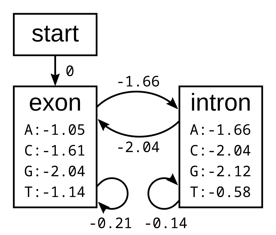
To demonstrate the backward algorithm, we will use the same example sequence CGGTTT and the same HMM as for the Viterbi and forward algorithm. Here again is the HMM with log emission and transmission probabilities:

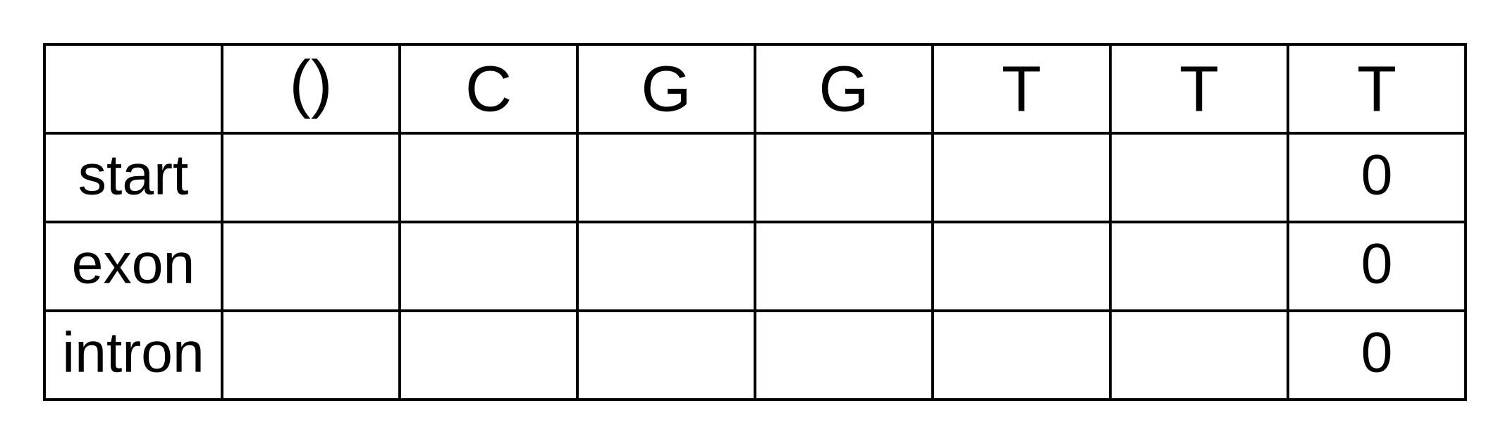
To calculate the backward probabilities, initialize a matrix b of the same dimensions as the corresponding Viterbi or forward matrices. The conditional probability of an empty sequence after the last position is 100% (or a log probability of zero) regardless of the state at the last position, so fill in zeros for all states at the last column:

To calculate the backward probabilities for a given hidden state k at the second-to-last position i = n - 1, gather the following log probabilities for each hidden state k’ at position i + 1 = n:

1. the hidden state transition probability t_k,k’ from state k at i to state k’ at i + 1
2. the emission probability e_k’,i+1 of the observed state (character) at i + 1 given k’
3. the probability b_k’,i+1 of the sequence after i + 1 given state k’ at i + 1

The sum of the above log probabilities gives us the log joint probability of the sequence from position i + 1 onwards and the hidden state at i + 1 being k’, conditional on the hidden state at i being k. The log sum of exponentials (LSE) of the log joint probabilities for each value of k’ marginalizes over the hidden state at i + 1, therefore the result of the LSE function is the log conditional probability of the sequence alone from i + 1.

We do not have to consider transitions to the start state, because (1) these transitions are not allowed by the model, and (2) there are no emission probabilities associated with the start state. The only valid transition from the start state at the second-to-last position is to an exon state, so its log probability will be:

• b_start,n-1 = t_start,exon + e_exon,n + b_exon,n = 0 + -1.14 + 0 = -1.14

For the exon state at n - 1, we have to consider transitions to the exon or intron states at n. Its log probability will be the LSE of:

• t_exon,exon + e_exon,n + b_exon,n = -0.21 + -1.14 + 0 = -1.35
• t_exon,intron + e_intron,n + b_intron,n = -1.66 + -0.58 + 0 = -2.24

The LSE of -1.35 and -2.24 is -1.01. and and For the intron state at n - 1 the log-probabilities to marginalize over are:

• t_intron,exon + e_exon,n + b_exon,n = -2.04 + -1.14 + 0 = -3.18
• t_{intron,intron} + e_intron,n + b_intron,n = -0.14 + -0.58 + 0 = -0.72

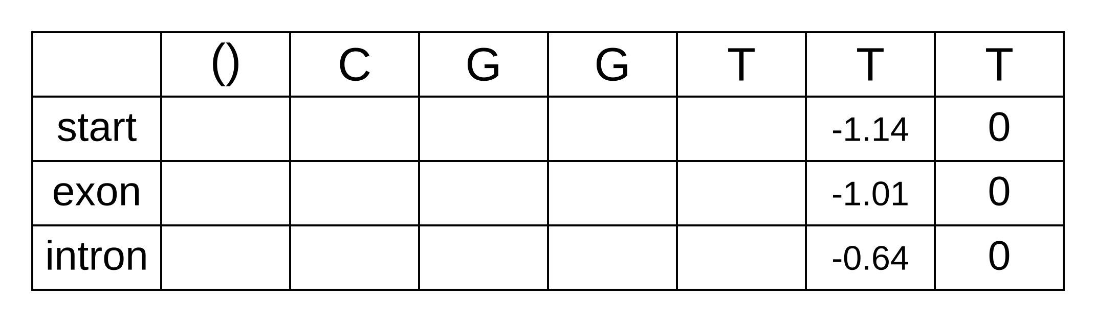
The LSE of -3.18 and -0.72 is -0.64. We can now update the backward matrix with the second-to-last column:

The third-to-last position is similar. For the start state we only have consider the one transition permitted by the model:

• b_start,n-2 = t_start,exon + e_{exon,n - 1} + b_{exon,n - 1} = 0 + -1.14 + -1.01 = -2.15

For the exon state at n - 2, the same as for n - 1, we have to consider two log-probabilities:

• t_exon,exon + e_{exon,n - 1} + b_{exon,n - 1} = -0.21 + -1.14 + -1.01 = -2.36
• t_exon,intron + e_{intron,n - 1} + b_{intron,n - 1} = -1.66 + -0.58 + -0.64 = -2.88

The LSE for these log probabilities is -1.89. Likewise for the intron state at n - 2:

• t_intron,exon + e_{exon,n - 1} + b_{exon,n - 1} = -2.04 + -1.14 + -1.01 = -4.19
• t_{intron,intron} + e_{intron,n - 1} + b_{intron,n - 1} = -0.14 + -0.58 + -0.64 = -1.36

And the LSE for these log probabilities is -1.30. We can now fill in the third-to-last column of the matrix, and every column going back to the first column of the matrix:

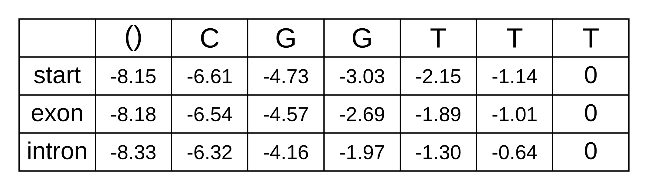
The first column of the matrix represents the beginning of the sequence, before any characters have been observed. The only valid hidden state for the beginning is the start state, and therefore the log probability b_start,0 = logP(x_1..n|π₀=start,M) can be simplified to logP(x_1..n|M). Because the sequence from 1 to n is the entire sequence, it can be further simplified to logP(x|M). In other words, this value is our log marginal likelihood! Reassuringly, it is the exact same value we previously derived using the forward algorithm.

Why do we need two dynamic programming algorithms to compute the marginal likelihood? We don’t! But by combining probabilities from the two matrices, we can derive the posterior probability of each hidden state k at each position i, marginalized over all paths through k at i. How this this work? If two variables a and b are independent, their joint probability P(a,b) is simply the product of their probabilities P(a) × P(b). Under our model, the two segments of the sequence x_1..i and x_i+1..n are dependent on paths of hidden states. However, the because we are using a hidden Markov model, the path and sequence from i onwards depends only on the particular hidden state at i. This is because the transition probabilities are Markovian so they depend only on the previous hidden state, and because the emission probabilities depend only on the current hidden state. As a result, while P(x_1..i|M) and P(x_i+1..n|M) are not independent, P(x_1..i|π_i=k,M) and P(x_i+1..n|π_i=k,M) are! Therefore (dropping the model term M for space and clarity):

P(x_1..i|π_i=k) × P(x_i+1..n|π_i=k) × P(π_i=k) = P(x_1..i, x_{i + 1..n}|π_i=k) × P(π_i=k) = P(x|π_i=k) × P(π_i=k)

Using the transitivity of equivalence, the product on the left hand side above must equal the product on the right hand side above. By applying the chain rule, it can also be shown that both are equal to the product on the right hand side below:

P(x|π_i=k) × P(π_i=k) = P(x_1..i|π_i=k) × P(x_i+1..n|π_i=k) × P(π_i=k) = P(x_1..i, π_i=k) × P(x_i+1..n|π_i=k)

Or in log space:

logP(x|π_i=k) + logP(π_i=k) = logP(x_1..i, π_i=k) + logP(x_i+1..n|π_i=k)

Notice that the sum on the right hand side above corresponds exactly to f_k,i + b_k,i! Now using Bayes rule, and remembering that b_start,0 equals the log marginal likelihood, we can calculate the log posterior probability of π_i=k:

logP(π_i=k|x) = logP(x|π_i=k) + logP(π_i=k) - logP(x) = logP(x_1..i, π_i=k) + logP(x_i+1..n|π_i=k) - logP(x) = f_k,i + b_k,i - b_0,start

And now we can now “decode” our posterior distribution of hidden states. We need to refer back to the previously calculated forward matrix, shown below.

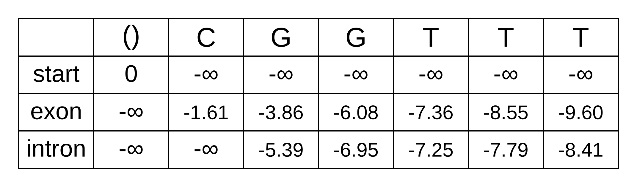
As an example, let’s solve the log marginal probability that the hidden state of the fourth character is an exon:

logP(π₄=exon|x,M) = f_exon,4 + b_exon,4 - b_start,0 = -1.89 + -7.36 - -8.15 = -1.1

The marginal probability is exp(-1.1) = 33%. Since we only have two states, the probability of the intron state should be 67%, but let’s double check to make sure:

logP(π₄=intron|x,M) = f_intron,4 + b_intron,4 - b_start,0 = -1.30 + -7.25 - -8.15 = -0.4

Since exp(-0.4) = 67%, it seems like we are on the right track! The posterior probabilities can be shown as a graph in order to clearly communicate your results:

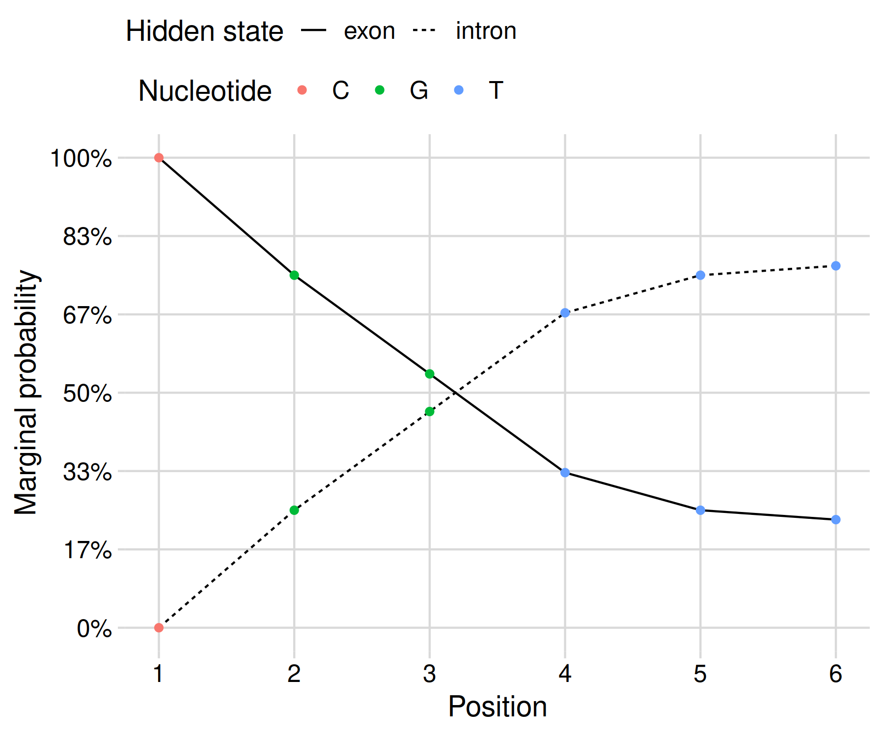
This gives us a result that reflects the uncertainty of our inference given the limited data at hand. In my opinion, this presentation is more honest than the black-and-white maximum a posteriori result derived using Viterbi’s algorithm.

For another perspective on the backward algorithm, consult lesson 10.11 of Bioinformatics Algorithms by Compeau and Pevzner.