Forward algorithm

The Viterbi algorithm identifies a single path of hidden Markov model (HMM) states. This is the path which maximizes the joint probability of the observed data (e.g. a nucleotide or amino acid sequence) and the hidden states, given the HMM (including transition and emission frequencies).

Maybe this path is almost certainly correct, but it also might represent one of many plausible paths. Putting things quantitatively, the Viterbi result might have a 99.9% probability of being the true¹ path, or a 0.1% probability. It would be useful to know these probabilities in order to understand when our results obtained from the Viterbi algorithm are reliable.

Recall that the joint probability is P(π,x|M) where (in the context of biological sequence analysis) x is the biological sequence, π is the state path, and M is the HMM. Following the chain rule, this is equivalent to P(x|π,M) × P(π|M). The maximum joint probability returned by the Viterbi algorithm is therefore the product of the likelihood of the sequence given the state path, and the prior probability of the state path! Previously I have described the product of the likelihood and prior as the unnormalized posterior probability. The parameter values which maximize that product, and therefore the state path returned by the Viterbi algorithm, is often known as the “maximum a posteriori” solution.

The posterior probability is obtained by dividing the unnormalized posterior probability (which can be obtained using the Viterbi algorithm) by the marginal likelihood. The marginal likelihood can be calculated using the forward algorithm.

The intermediate probabilities calculated using the Viterbi algorithm are the probabilities of a state path π and a biological sequence x up to some step i: P(π_1..i,x_1..i|M). The intermediate probabilities calculated using the forward algorithm are similar but marginalize over the state path up to step i: P(π_i,x_1..i|M). Put another way, the probability is for the state at position i integrated over the path followed to that state.

This marginalization is achieved by summing over the choices made at each step. When calculating probabilities, summing typically achieves the result of X or Y (e.g., a high OR low path), whereas a product typically achieves the result of X and Y (e.g. a high then low path).

Just as for the Viterbi algorithm, it is sensible to work in log space to avoid numerical underflows and loss of precision. As an alternative to working in log space while still avoiding those errors, the marginal probabilities of all states at any position along the sequence can be rescaled (see section 3.6 of Biological Sequence Analysis). However if those marginal probabilities are very different in magnitude, there can still be numerical errors even with rescaling, so from here on we will work in log space.

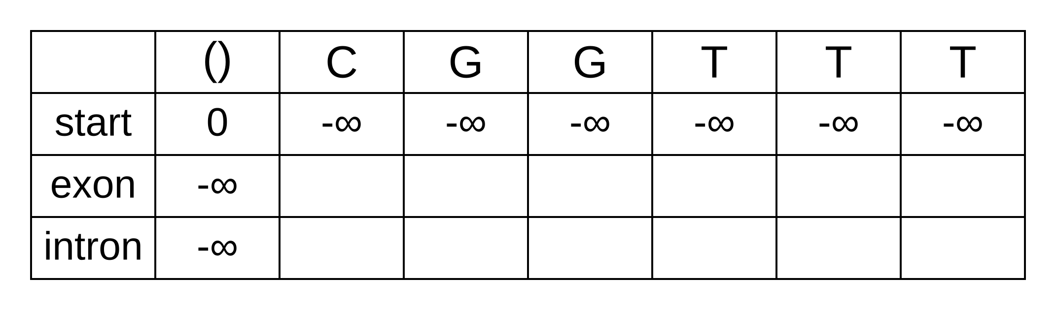
As an example we will use the forward algorithm to calculate the log marginal likelihood of the sequence CGGTTT and HMM used in the Viterbi example. Initialize an empty forward matrix with the first row and column filled in, same as the Viterbi matrix:

To calculate the log marginal probability of a particular state at some position of the sequence, we need to sum over the probabilies that lead from any previous state to the particular state at that position. These are not the log-probabilities being summed over, but the actual zero to one probabilities. In log space, this requires logging the sum of exponentials of the log-probabilities, or LogSumExp (LSE) for short.

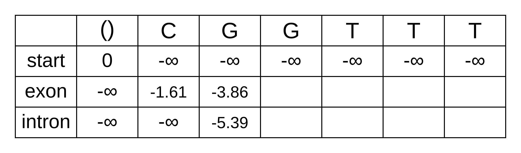
The only valid paths up to the second position of the sequence under our model are start-exon-exon and start-exon-intron, so the first three columns will be identical to the Viterbi matrix as no summation is required:

Because of the marginalization, there are no pointer arrows to add to the forward matrix. The third position (fourth column) is more interesting, as we have to marginalize over multiple log probabilities of the state at the previous position. For the exon state at the third position, these log probabilities are:

• f_exon,2 + t_exon,exon + e_exon,3 = -3.86 + -0.21 + + -2.04 = -6.11
• f_intron,2 + t_intron,exon + e_exon,3 = -5.39 + -2.04 + -2.04 = -9.47

The log marginal probability (to two decimal places) is therefore LSE(-6.11, -9.47) = log(exp(-6.11) + exp(-9.47)) = -6.08. This calculation can be performed in one step using the Python function scipy.special.logsumexp. To use this command scipy must be installed and the scipy.special subpackage must be imported. In fact, it should be performed in one step to avoid the aforementioned numerical errors.

The log probabilities to marginalize over for the intron state at the third position are:

• f_exon,2 + t_exon,intron + e_intron,3 = -3.86 + -1.66 + -2.12 = -7.64
• f_intron,2 + t_{intron,intron} + e_intron,3 = -5.39 + -0.14 + -2.12 = -7.65

The log marginal probability is therefore LSE(-7.64, -7.65) = log(exp(-7.64) + exp(-7.65)) = -6.95. The log marginal probabilities for each state at each position can be calculated the same way, and the completed forward matrix will be:

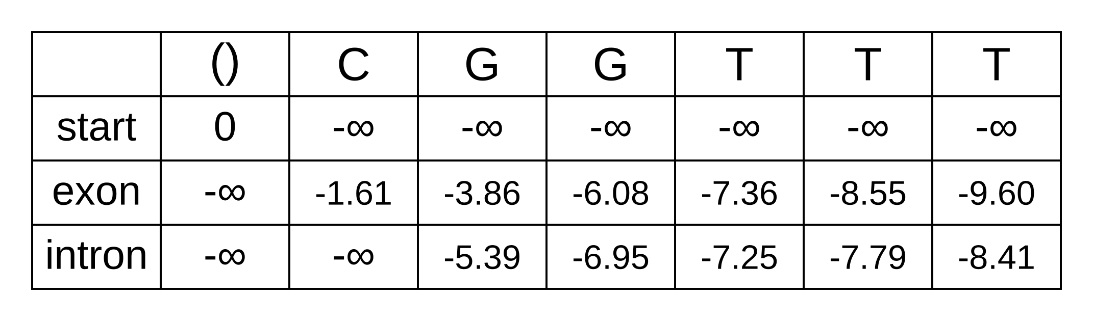
At the last position, we have the log marginal joint probability of the sequence and path over all paths that end in an exon state, and log marginal joint probability over all paths that end in an intron state. The LSE of these two log probabilities is therefore the log marginal likelihood of the model, because it marginalizes over all state paths, and equals to LSE(-9.60, -8.41) = log(exp(-9.60) + exp(-8.41)) = -8.15.

We previously calculated the log probability of the maximum a posteriori path as -9.79. The posterior probability is therefore exp(-9.79 - -8.15) = exp(-1.64) = 19.4%. The Viterbi result is very plausible (events with 19.4% probability occur all the time) but most likely wrong.

For more information see section 3.2 of Biological Sequence analysis by Durbin, Eddy, Krogh and Mitchison.

For another perspective on the forward algorithm, consult lesson 10.7 of Bioinformatics Algorithms by Compeau and Pevzner.

1. Such probabilities are conditioned on the model being correct. So more accurately, they are the probability of a parameter value being true if the model (e.g. an HMM) used for inference is also the model which generated the data. If the model is wrong, the probabilities can be quite spurious, see Yang and Zhu (2018). ↩