PAM (Dayhoff) matrices

The point accepted mutation (PAM) substitution model, also known as the Dayhoff substitution model, is an amino acid substitution model derived from empirical observation of mutations among closely related proteins. This venerable model was described in various volumes and supplements of the Atlas of Protein Sequence and Structure, with the most well-known version being published in the 1978 supplement by Dayhoff, Schwartz and Orcutt.

Since 1966, Dayhoff and her colleagues had been collecting and compiling protein sequences into their Atlas, and groups of closely related sequences from the Atlas were used as the basis for the PAM matrix. Where more than two sequences were in a group, phylogenetic trees were inferred along with ancestral sequences on each node of the tree, presumably using a method similar to the one published by Eck and Dayhoff in 1966. This method has been variously described as maximum parsimony (e.g. in Zhang and Nei 1996) or minimum evolution (e.g. in Edwards 1996).

Maximum parsimony (MP) methods optimize for the smallest possible number of mutations; for a given tree there will be a minimum number of mutations required to explain the known sequences, and MP methods attempt to find the tree with the smallest minimum number of mutations.

Each branch of a tree is associated with a pair of sequences, one at either end of the branch. These pairs of sequences were extracted from each tree. For each pair of sequences either from a tree or from the groups of size two, if there were two different amino acids at a given position it was assumed that a single mutation - a PAM - had occured, directly changing the amino acid of one of the sequences to the amino acid of the other sequence. This assumption is justified on the basis that sequences will be closely related enough that only one or zero mutations are likely to have occured at each site within these pairs. Models of sequence evolution making this assumption are commonly known as infinite-sites models (e.g. in Tajima 1996). If this assumption holds, then the vector of counts of mutations from one amino acid to the other nineteen amino acids should be proportional to the rates of transition from that one amino acid to the other nineteen, albeit with some sampling error.

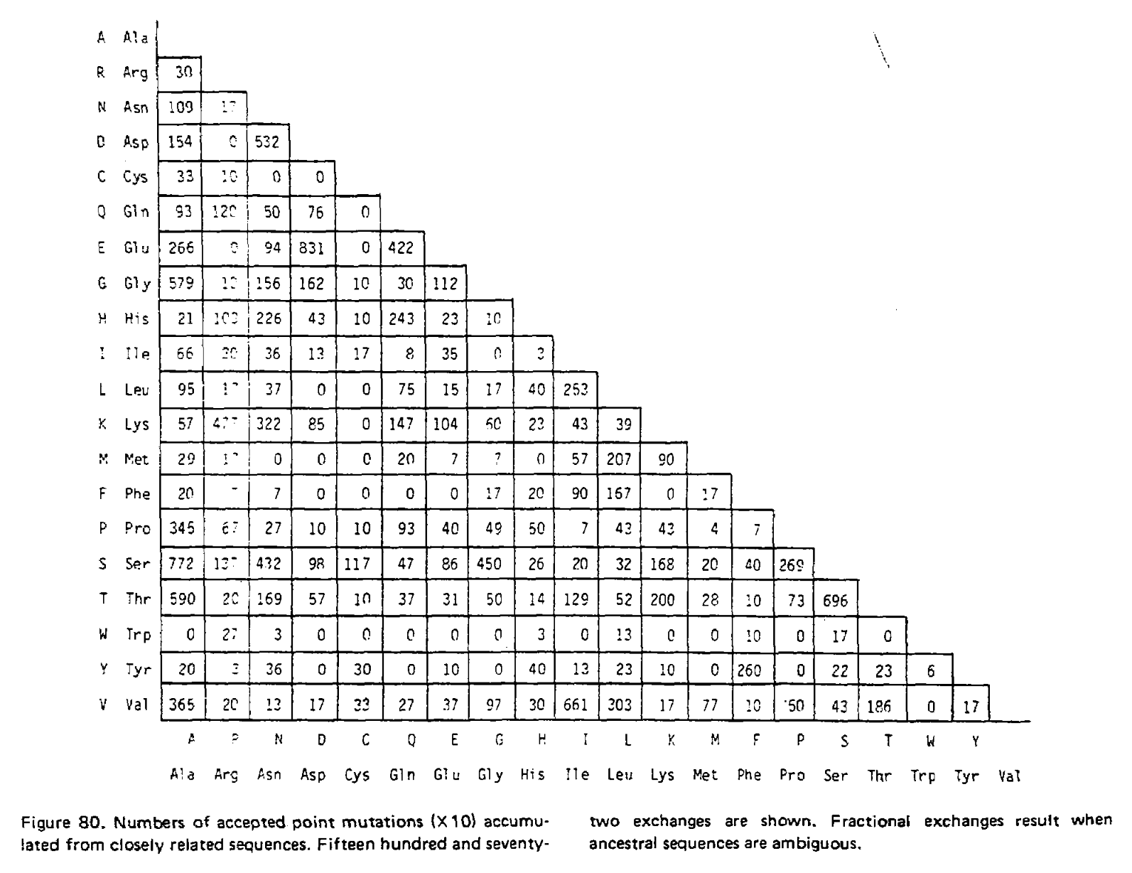
In the 1978 version of the matrix, 71 groups were identified containing 1,572 mutations in total. Using the above procedure, point accepted mutations occuring in this dataset were counted and recorded in a matrix called A. This is a triangular matrix because the process is assumed to be reversible conditional on there being a mutation from the initial state; the probability of a mutation from state X to state Y, conditional on there being a mutation from state X to anything else, is the same as a mutation from Y to X conditional on there being a mutation from Y to anything else. Here is the count matrix:

We want to transform this matrix into a transition probability matrix M. Given some alphabet of states C, that matrix gives us the probability of a particular end state C_i (in this case, a particular amino acid) given an initial state C_j and some duration of time t, which we can write as M_ij = P(C_i|C_j, t). For the case where a mutation has definitely occured and i is different from j, we can express this as the joint probability P(C_i, i ≠ j|C_j, t), which will correspond to the off-diagonal elements of M. Following the chain rule, we can decompose this joint probability into P(C_i|C_j, i ≠ j, t)P(i ≠ j|C_j, t). When t is small enough that the infinite sites assumption is reasonable, then the probability of C_i conditioned on i ≠ j will not depend on t, and this formulation can be approximated as P(C_i|C_j, i ≠ j)P(i ≠ j|C_j, t).

We can estimate P(C_i|C_j, i ≠ j) from the symmetric version of the above triangular matrix of counts, by transforming the count of j to i mutations A_ij into a proportion by dividing this count by the total number of all mutations starting with j, or Σ_iA_ij. To compute the probability of any mutation P(i ≠ j|C_j, t), first the relative “mutability” m of each amino acid was calculated, a value which is proportional to (but not equal to) that probability when t is small enough that multiple mutations are unlikely. Put another way, m_j is approximately proportional to P(i ≠ j|C_j, t) for any small value of t. To derive the PAM/Dayhoff matrix, mutability was estimated as the number of mutations involving C_j relative to the overall occurance of C_j across all sequences. This mutability score was normalized so that the mutability of alanine equaled 100, an arbitrary choice given m is only proportional to the desired probabilities.

Finally, for each amino acid, an overall scaling factor λ was used to scale m_j from a relative value to the probability of mutation given 1 unit of time, i.e. λm_j = P(i ≠ j|C_j, t = 1). We can now calculate the off-diagonal values (where i ≠ j) of the transition probability matrix for t = 1 as:

This scaling factor was calculated to set the unconditional mutation probability, that is P(i ≠ j), to equal 0.01 mutations per site, or equivalently equal 1 mutation for every 100 sites, given the resulting substitution matrix and an underlying amino acid frequency distribution. As a result, 1 unit of time is equal to the amount of time in which we expect 0.01 mutations to occur per site, which is called 1 PAM unit. Since whether or not a mutation has occured is a binary choice, the diagonal matrix values for 1 PAM unit, which correspond to P(i = j|C_j, t = 1), are equal to 1 - P(i ≠ j|C_j, t = 1) or:

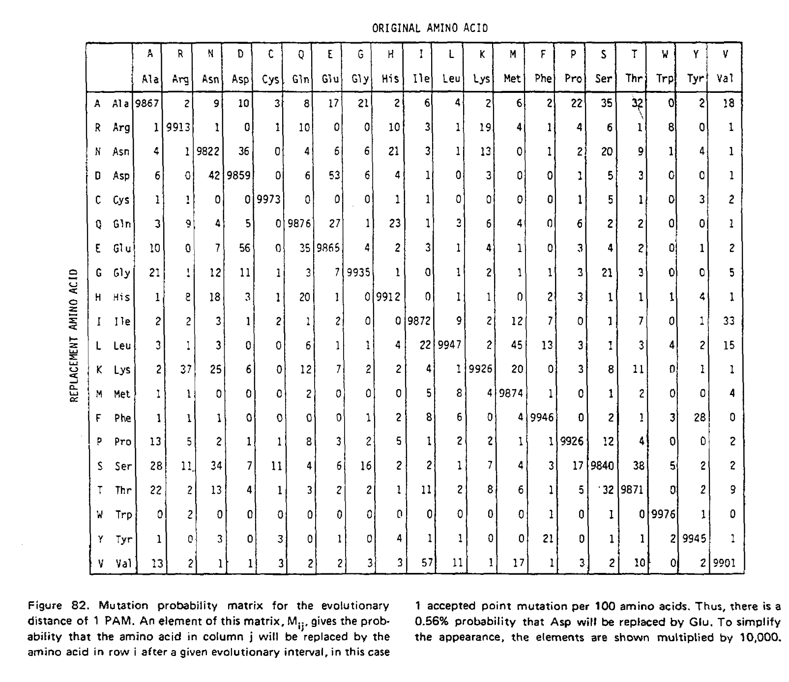
Using these two formulae, Dayhoff and colleagues calculated the entire transition probability matrix for 1 PAM unit:

However, it is unlikely we are analyzing sequences exactly 1 PAM unit apart. As such we need to derive matrices for greater values of t, and in their 1978 supplement Dayhoff and colleagues derived the PAM250 matrix. This was done using matrix multiplication because at larger distances, multiple substitutions become much more likely. To illustrate the use of matrix multiplication to derive PAMn matrices, let’s consider a toy example with just three states; red, green and blue. Here is our transition probability matrix for one time unit:

	red	green	blue
red	0.95	0.08	0.01
green	0.04	0.84	0.04
blue	0.01	0.08	0.95

While modern phylogenetic methods treat evolution as a continuous-time Markov chain (CTMC) where each time step is infinitesimally small, in this case I will approximate evolution as a discrete-time Markov chain (DTMC) with time steps of 1 time unit as it is easier to explain.

After one time step, there is only one way a state can remain unchanged; no mutation must have occured. But after two time steps there is another possibility; a mutation occured at the first time step, and was reversed in the second.

For example, if the state is red at the start and end of the process, it could have remained unchanged over two time steps, but could also have mutated to green in the first time step and back to red, or to blue and back. We therefore need to sum over these possibilities to get the probability of remaining red over two time units. We calculate this sum as M₁₁×M₁₁ + M₁₂×M₂₁ + M₁₃×M₃₁ = 0.95×0.95 + 0.04×0.08 + 0.01×0.01 = 0.9058. The same logic applies to every other entry in our matrix, and we can use it to create a the transition probability matrix for two time units:

	red	green	blue
red	0.9058	0.1440	0.0222
green	0.0720	0.7120	0.0720
blue	0.0222	0.1440	0.9058

We have just performed matrix multiplication, calculating M×M=M²! We could multiply the resulting matrix by M again to get M³, the transition probability matrix for three time units. The PAMn matrices were calculated this way, for example the PAM250 matrix:

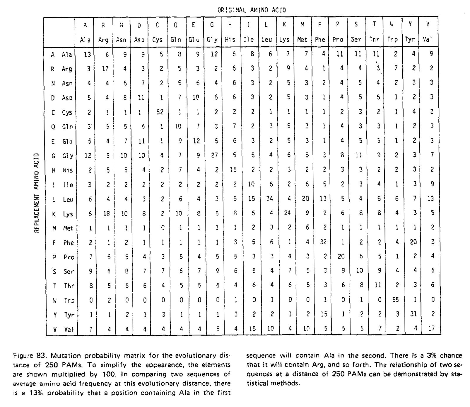
Notice how the transition probabilities get “flatter” the more time has passed. Given an infinite amount of time, each column would have an identical set of probabilities; the final amino acid would be completely independent of the initial amino acid, and the log-odds scores calculated from these transition probabilities would be identical to the non-homologous log-odds scores.