BLAST and FASTA

Pure Smith–Waterman is unpopular because of its poor scaling. Given two sequences of unequal lengths n and m, we have to compute nm intermediate values. We therefore consider the algorithm to run in O(nm) time, or O(n²) time for sequences of roughly equal length n.

For example, if you have a 1000nt long RNA molecule to align with a 100 megabase chromosome, there will be one hundred billion intermediate calculations to perform.

The popular local aligners FASTA and BLAST both introduce heuristics, based on k-mer matches between the query and database sequences, to minimize the Smith–Waterman search space. k-mers are sequence “words” of fixed length k, so for example a peptide sequence 20 amino acids long is called a 20-mer.

These heuristics attempt to exchange a small decrease in accuracy for a large increase in speed. For both methods there are parameters that may be adjusted to modify this trade-off. The first step of both FASTA and BLAST is to create a hash table of all the k-mers in the query sequence. The k-mer length k is a tunable parameter for both methods.

BLAST has another parameter T (for Threshold), where any similar k-mer with a global alignment score against the original k-mer of at least T will also be stored in the hash table. This allows for inexact matches with the original query sequence at the k-mer level. Lower values of T will improve accuracy at the expense of speed, as more k-mers will match and more local alignments dynamically generated.

Hash tables provide a way to very quickly check whether a k-mer is present in the query, and if so the matching positions in the query. Imagine that the query sequence Q is HMERMIKIHHQELGCCIIWT. There are 10 unique 10-mers within this sequence, the first beginning at position 0, the second at position 1 and so on. Looking up the value at a specific location in memory is extremely fast, so the most obvious way to quickly lookup k-mers is to convert them into integers, and store their position in RAM at the location corresponding to its integer.

For amino acids there are 20¹⁰ possible 10-mers, which equals 10,240,000,000,000 (10 trillion). If we use 1 byte to store the position of each k-mer within the query sequence, our lookup table would require 10 terabytes of RAM! Even in 2018 this is an uncommon amount of memory.

Instead we can use a hash function to generate a relatively small integer from some original value, in this case from the k-mer string. A simple way to do this for k-mers is to use an integer based on the first sequence character. Based on the standard protein alphabet ARNDCQEGHILKMFPSTWYV, we can use 0 for A, 1 for R, 2 for N and so on.

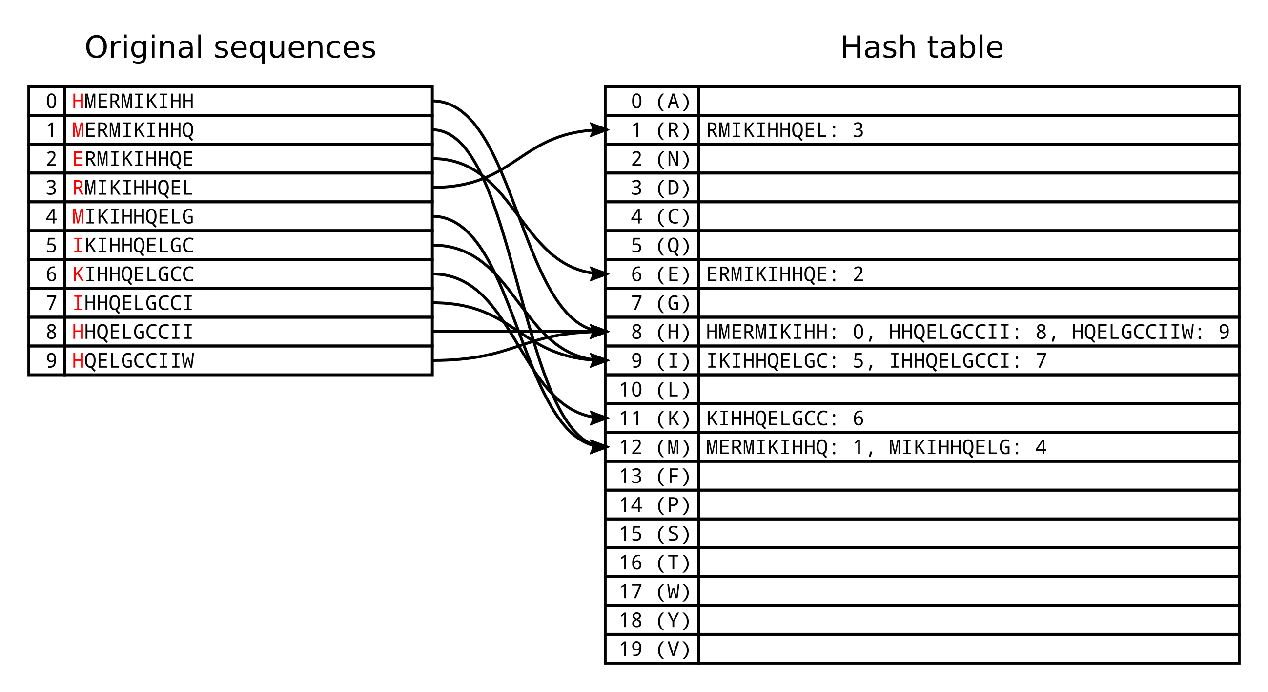
In this case we would have 20 buckets (also known as cells or slots) in our hash table. However multiple unique k-mers will by chance have the same hash function result, and will therefore be assigned to the same bucket. The load factor of the hash table is the number of entries divided by the number of buckets. In the above example the load factor is 0.5, because there is on average 0.5 entires in each bucket.

When running BLAST or FASTA, we scan each position in the database (or target) sequences by hashing the k-mer at that position and checking the hash table for corresponding k-mers. If the load factor of the hash table is too high, we will have to spend more time checking each k-mer in the bucket for a match.

We can decrease the load factor by changing our hash function to generate longer hash values. For example we could use the first two letters of the k-mers, which would require 20² = 400 buckets. However if our hash values are too long, the number of buckets might exceed the available memory in a computer and the program will crash.

This is a classic example of a space-time trade-off, where we can use up more memory (space) in exchange for better performance (time). In the best case scenario, finding all k-mer matches between query and target sequences will take O(n) time, where n is the length of the target or database.

After identifying exact k-mer matches, FASTA then identifies the 10 best diagonal regions based on the density of k-mer matches. Next, the combination of compatible diagonal regions with the best ungapped alignment scores is determined. Diagonal regions are gapless alignments, are two regions are compatible if there is no overlap between their X sequences or their Y sequences. Finally a banded Smith–Waterman search is undertaken, centered on the compatible regions.

Let’s take an example from the CLV1 and CLV2 sequences. The 6-mer LTGSIP is preserved between the two sequences, so we can conduct a banded Smith–Waterman search by restricting the search to four cells in any direction (up, down, left or right) from the diagonal:

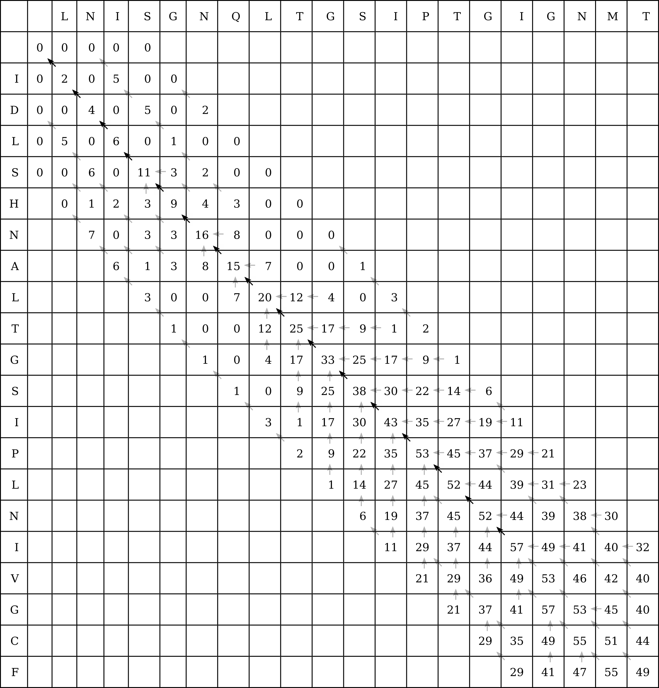
Of course if the band is too narrow, there may be enough gaps in one of the sequences for the optimal local alignment to lie outside of this band (without gaps in the other sequence to pull it back inside the band before it drifts outside), and then FASTA will be less accurate than a full Smith–Waterman search.

This heuristic doesn’t make much difference in this example where we have only two 20 character long sequences, or 400 intermediate calculations to perform. We still had to calculate 160 intermediate values, or 40% of the original number. However in the original example of a 1000nt long RNA molecule aligned to a 100 megabase genome, banded Smith–Waterman will eliminate almost all of the intermediate values.

Gapped BLAST uses quite different heuristics from FASTA. Its two-hit method identifies potentially homologous regions (high-scoring segment pairs, or HSPs) by checking for non-overlapping but close k-mers which lie on the same diagonal in the query and in the database.

The central residue pair of whatever 11 contiguous pairs of residues within the HSP has the highest alignment score is used as a seed residue. From this seed residue, the Smith–Waterman algorithm is run in the forward (N terminus to C terminus, or 5’ to 3’ for DNA) and separately in the reverse (C to N, or 3’ to 5’) direction.

Because the seed residue pair is assumed to be part of the optimal local alignment, once the score reaches zero in some cell, calculation of alignment scores is unnecessary beyond that cell. This is because any local alignments that begin after that cell will not include the seed residue pair.

See in this alignment of two proteins from Altschul et al. (1997) how using the seed residue pair to initialize forward and reverse searches greatly limits the local alignment search space:

The forward search is in the top right hand corner, the reverse search is below and to the left of that. The black cells show where the values in the Smith–Waterman matrix are positive and contiguous with the seed pair.

Of course if the seed residue pair is not actually homologous and/or not part of the optimal local alignment, the method will be inaccurate. For more information on FASTA, see the publication from Pearson and Lipman (1998). For more information on BLAST, see the publication from Altschul et al. (1997) on gapped alignment in BLAST.