Priors and clock models in StarBEAST2 tutorial

Step 0: Download the example data set

The following programs should already be installed:

• BEAST 2
• BEAUti 2
• DensiTree
• StarBEAST 2
• Tracer

The first three come with the BEAST 2 package. StarBEAST2 is an add-on for BEAST 2. Tracer is a separate program from BEAST 2, and can be used to inspect the output of any Bayesian program that uses the MCMC algorithm.

Download the example archive. This is a collection of multiple sequence alignments from species of Canis and closely related genera. After downloading the archive, extract it somewhere.

Step 1: Open the StarBEAST2 template

Open “BEAUti” (in the BEAST2 folder), which is a GUI application for configuring a BEAST2 analysis. Now select the StarBEAST2 template for multispecies coalescent analyses:

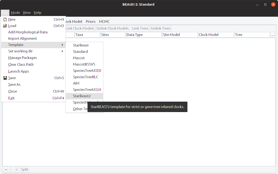
The title bar should have changed to “BEAUti 2: StarBeast2”

Step 2: Import multiple sequence alignments

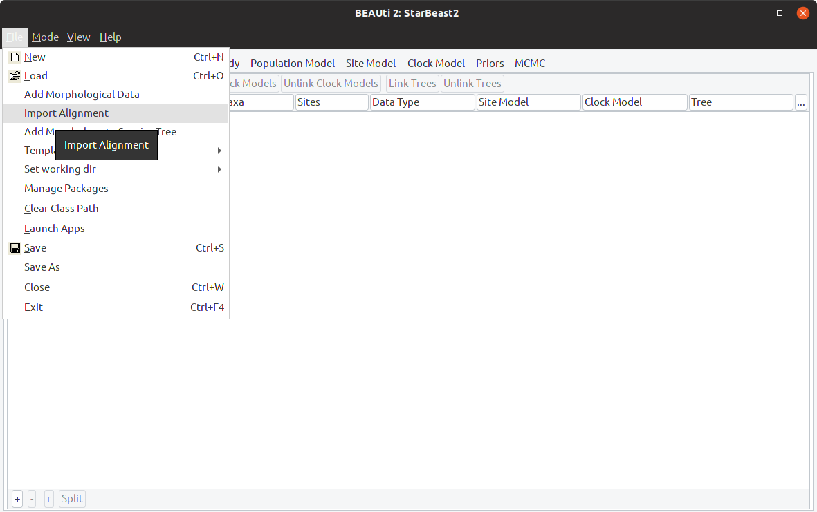
Now import the multiple sequence alignments you previously downloaded and extracted. Either click the plus button in the bottom left, or use the Import Alignment menu item:

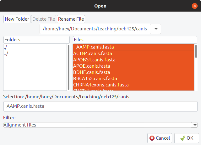
Each locus has its own fasta file in the example data set. Select all of the loci to import, then select “all are nucleotide” when asked to specify the datatype:

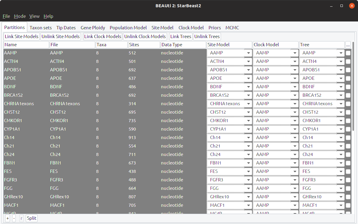
Step 3: Link clock models

All of the loci should appear in the main BEAUti window now. Select all of them, and choose to “Link Clock Models” using the button at the top. This will enable estimating a weighted average clock rate for all loci. After linking, all loci should be sharing the same clock model name:

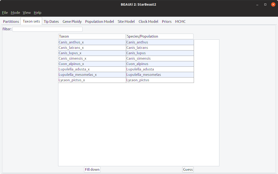
Step 3: Specify taxon sets

Open the “Taxon sets” tab. This is where the mapping between the names used for gene sequences and the names of species is constructed. Click the button labelled “Guess” and select “Before Last”:

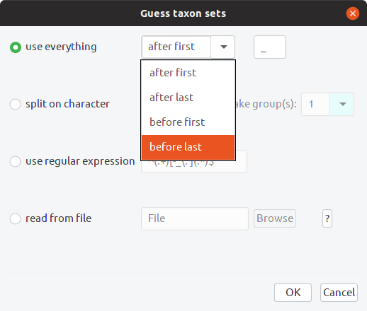
Click OK. Notice that the taxon names all had an “_x” on the end. This is because BEAST gets mad if the names of species and the names used for gene sequences are the same. Adding this suffix, and removing it in BEAUti to get the species names, is a way around that issue. Your taxon sets should look like this:

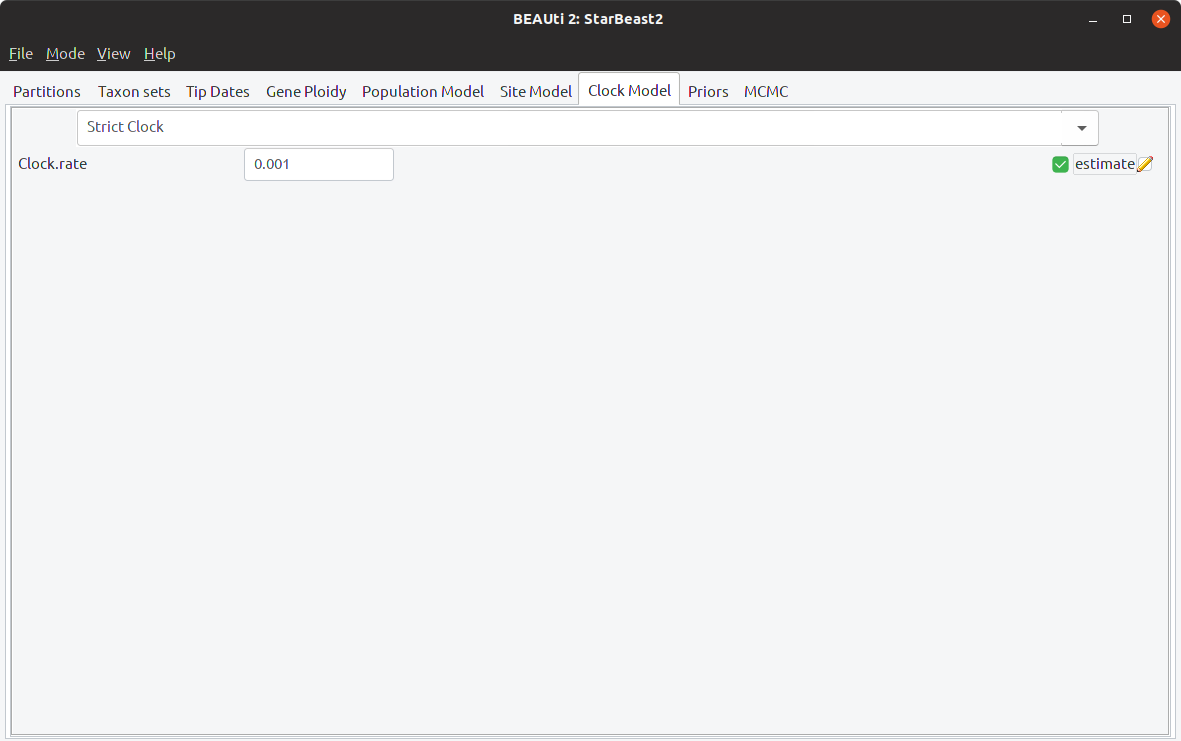
Step 4: Estimate the clock rate

Open the Clock Model tab, and enable “estimate” next to the clock rate. Change the rate to 0.001 - this is the initial value of the rate, and changing it to a value closer to the posterior mode will help our analysis to converge quickly. The Clock Model tab should now look like this:

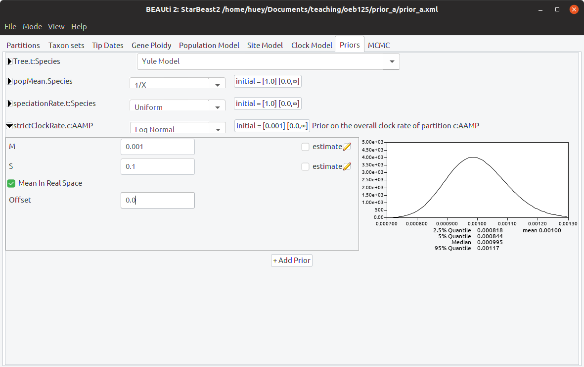
Step 5: Specify the clock rate prior

Go to the Priors panel, and expand the “strictClockRate” prior. Change the mean “M” to 0.001, and the standard deviation “S” to 0.1. The prior distribution on clock rate should now look like this:

Step 6: Save and launch

Save your configuration to a new folder, called something like “slow prior”. Launch BEAST, and open the configuration file you just created. Start the analysis, which will take 5 to 10 minutes to complete.

Step 7: Rinse and repeat

Repeat steps 1 through 6, but this time specify an initial clock rate of 0.01, and a clock rate mean “M” of 0.01. Use the same standard deviation “S” of 0.1. Make sure to save your new configuration file in a different folder, called something like “fast prior”.

Step 8: Interrogate the results using Tracer

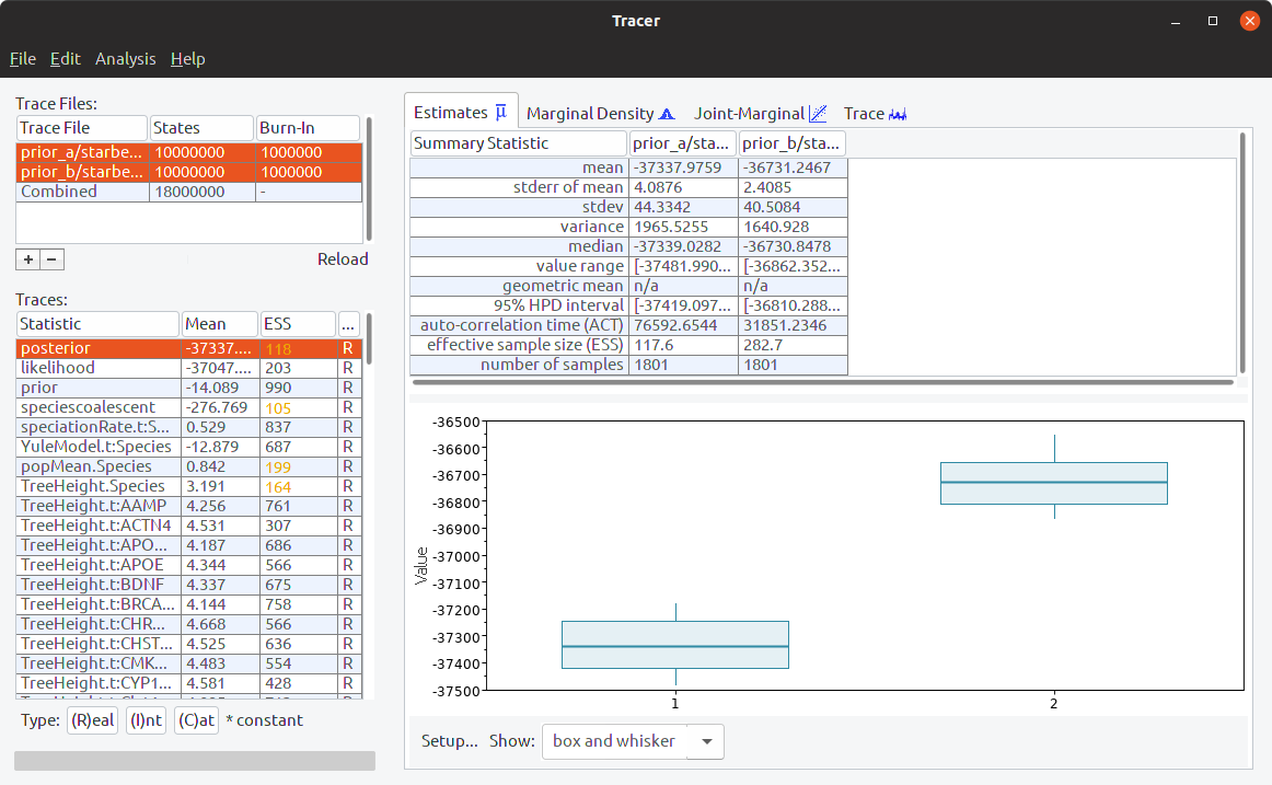
Open Tracer, and select Import Trace File from the file menu. Open the “starbeast.log” file from your “slow prior” folder. Then open the “starbeast.log” file from your “fast prior” folder in the same Tracer window. Highlight both trace files:

.

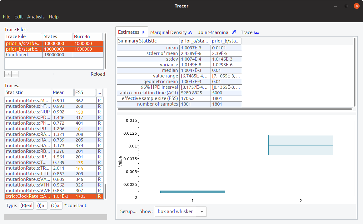
Select different statistics to see if their distributions are different between the analyses. In particular, look at the strictClockRate distributions (which should be the last statistic):

.

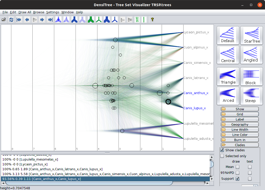
Step 9: Look at the trees in DensiTree

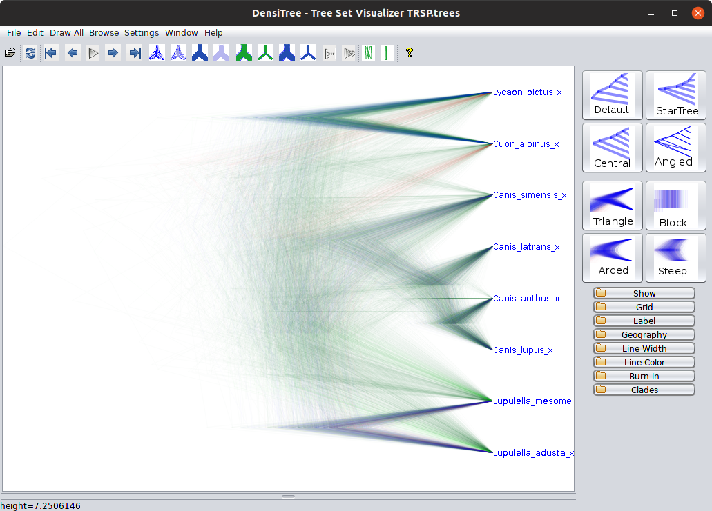
Once you are finished with Tracer, explore the different tree files for both analyses with DensiTree. The gene tree files are named based on the locus, and the species tree files are always called “species.trees”. For example, open the TRSP posterior distribution (\texttt{TRSP.trees}}) in DensiTree, and enable the “Full grid” so you can see the divergence times:

.

You can use DensiTree to calculate the posterior probability of clades. This is the probability that a group of sequences or species are monophyletic (share a single common ancestor to the exclusion of all other sequences or species in the data set), given the data set and the model. To do this is a little convoluted:

1. Select the “Central” display mode (it won’t work with the default).
2. Enable the “clade toolbar” by selecting “view clade toolbar” in the window menu.
3. Open the “Clades” “folder” on the right hand side and enable “Show clades”.

The size of each circle is somewhat proportional to the posterior probability of the corresponding clade, and the postion along the X-axis is the expectation of the age of that clade. Take a note of the posterior probability and heights of some of the clades, for example:

Now compare the clades you can see and their heights in this gene tree with the clades in the corresponding “fast prior” gene tree, and both the “fast” and “slow” species trees.