
Markov models
Markov processes model the change in random variables along a time dimension, and obey the Markov property. Informally, the Markov property requires that the conditional probability of the random variables at some future time stays the same whether it is conditioned on (1) the entire past history of the random variables up to and including the present or (2) the present values of the random variables alone. A more precise mathematical definition is given in Chapter 5 of Kai Lai Chung’s “Green, Brown and Probability”:
Λ is a Borel set taken from the Borel tribe generated from a random variable X from the present time t onwards. In order words, it is a set or interval which could include X at some point in time t’ ≥ t. In this definition, the probability of X being included in that set or interval at t’ will be the same whether it is conditioned on (left of the quality) the Borel tribe generated from X from time zero to the present or (right of the equality) the Borel tribe generated from X in the present.
Markov processes can be used for generative or predictive methods. The Markov property makes it easier to simulate data or infer probabilities based on a Markov model, as we can infer the probability of the state at some future time t’ from the state at the present time t, instead of having to consider all the state in the past up to the present.
The time dimension can be discrete or continuous, and the values of the random variables (the state) can also be discrete or continuous. All combinations of discrete or continuous time and state are commonly used in sequence analysis, as I will detail below:
Discrete space, discrete time
Many models of gene, protein and genome sequence structure operate over a discrete space, for example the four nucleotides, or the 20 amino acids, or the 64 codons in the standard genetic code. They also operate over a discrete time dimension, where time zero is the first site or residue or codon in a linear sequence, time one is the second site, and so on. The CpG island and splice site models we will look at are discrete space, discrete time Markov processes.
Discrete space, continuous time
As with models of sequence structure, models of sequence evolution necessarily operate over a discrete space, since there are four nucleotides, 20 amino acids, and 64 codons in the standard genetic code. However the time dimension is continuous.
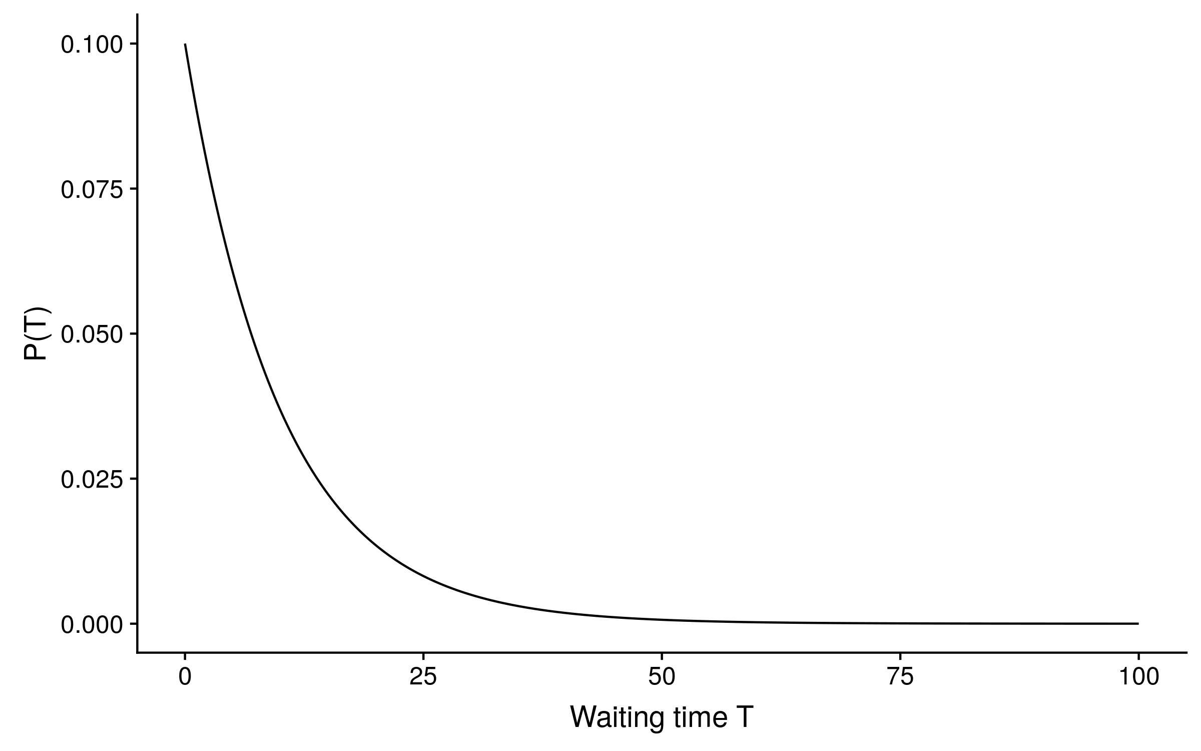
In the Jukes-Cantor model of sequence evolution, all transitions between states have equal probability, and the state frequencies are all equal, so there is only one parameter: the rate r of substitutions per unit of time. At each site in a sequence, the waiting time T for the next substitution to occur from any time t is modelled by an exponential distribution, which is continuous. If the Jukes-Cantor substitution rate is 0.1, the distribution of waiting time looks like this:
The exponential distribution is memoryless and so can be “reset” to begin at any time t and not change (as long as the rate r stays constant). In terms of sequence evolution, this means that if we observe an A nucleotide at t = 20, it will still be an A with some probability p at t = 40 (waiting time T = 20), and if it is still an A at t = 40, the probability that it is still an A at t = 60 (T = 20 again) will still equal p.
Because of this memorylessness, the Jukes-Cantor model (and many other models commonly used for sequence evolution) is Markovian; we can predict the future state probabilities from the observed state at some present time.
Continuous space, continuous time
If you are an physicist, then “Brownian motion” is the random movement of particles in a fluid medium like air or water, and is not necessarily Markovian. If you are a mathematician or a biologist, then “Brownian motion” is usually the continuous time limit of a Gaussian random walk process. The latter mathematical process is a simple way to model the former physical process.
The probability distribution of the difference between the state of a 1-dimensional random variable at time t and at time t+u is normally distributed with a mean of 0 and variance u. The time dimension is continuous, and the space is continuous as well, as the normal distribution is a continuous distribution.
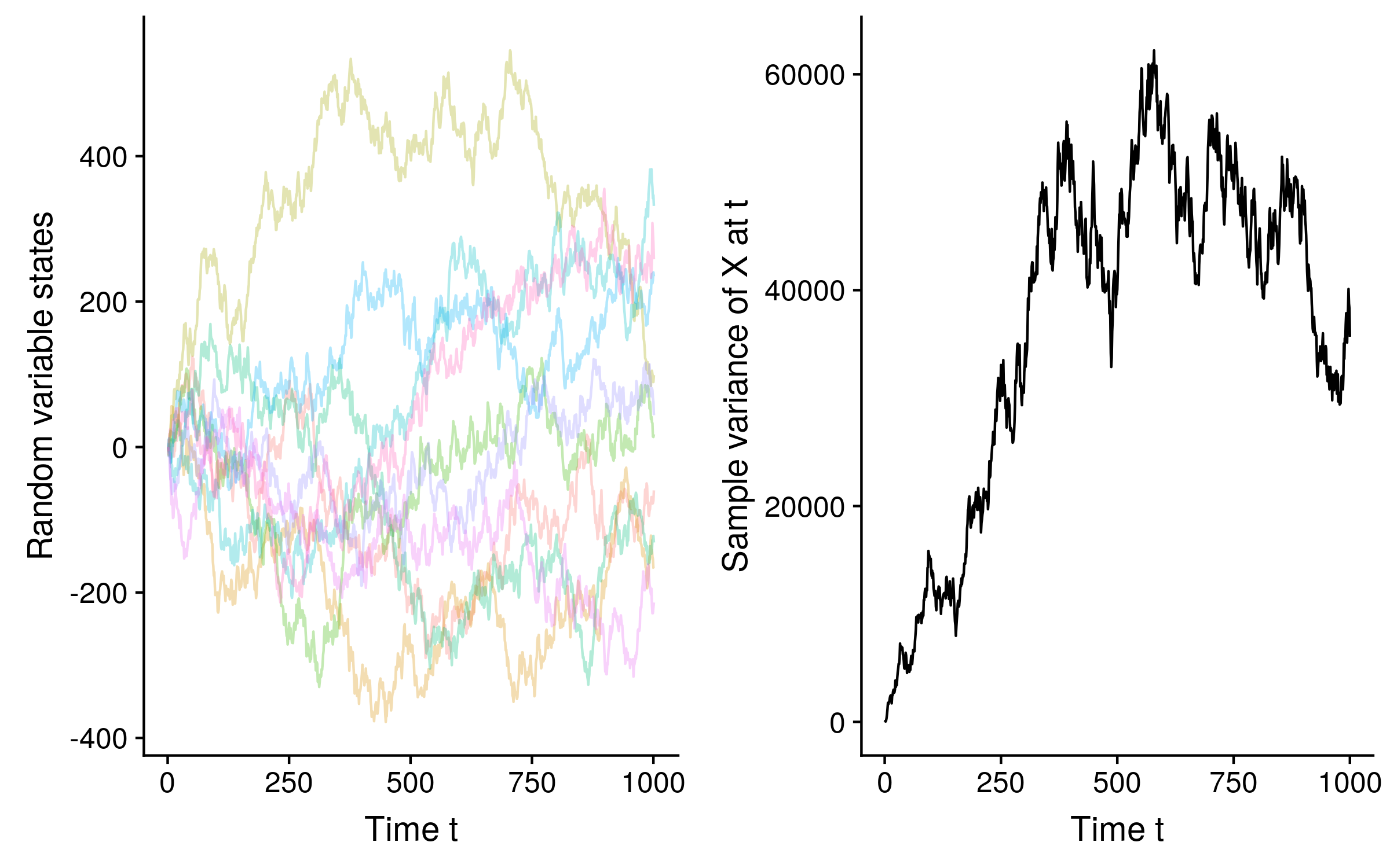
Since we can calculate the probability distribution of a random variable in the future from its state in the present, without reference to its entire past history, Brownian motion in the math/biology sense is Markovian, albeit non-stationary, in the sense that the probability distribution is not constant over time. See how the sample variance of 10 Brownian motion trajectories of a random variable X increases over time:
In fact unless we condition on observing the random variable state at some time t, the probability distribution of the random variable at any time t’ has infinite variance. Remember that under standard Brownian motion the probability distribution of Xt+u is N(Xt, u), so if u = ∞, the variance of x in the limit also equals ∞.
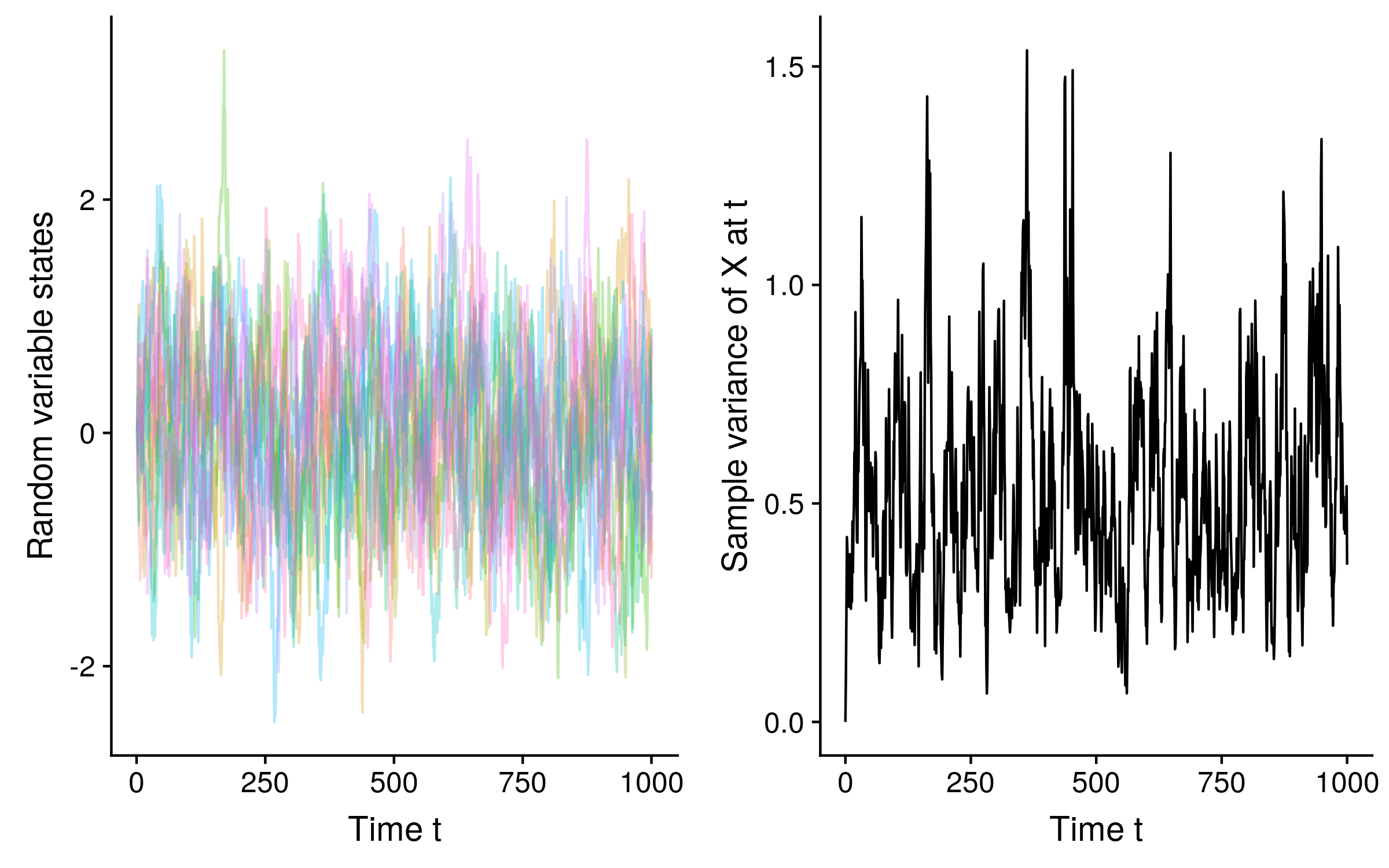
A similar process, the Ornstein-Uhlenbeck process (or the O-U process for short) is also Markovian. The difference between standard Brownian motion and O-U is that the random variable is biased towards reverting to a mean value. This means that unlike Brownian motion which is non-stationary, samples generated from an given O-U process over time approach a stationary distribution with a well defined mean and variance. See how the variance stabilizes over time for 10 O-U trajectories of a random variable X:
Continuous space, discrete time
Markov chain Monte Carlo (MCMC) is another Markovian process, and the indices of the iterations of an MCMC chain correspond to the times along a discrete time dimension. MCMC can be used to infer the posterior probabilities of discrete or continuous states. For example Faria et al. (2014) used MCMC to model the origin and spread of HIV along Congolese rivers and railways from 1920 to 1961:

The parameters estimated using MCMC included the time of introduction of HIV at each sample location above, and those times were used to generate the above figure. Note that the times of introduction are random variables and part of the space, and are not the time dimension in the context of Markov chain Monte Carlo!!! The time dimension is still the MCMC iterations, which remains discrete.
Phylogenetic studies tend to use either “coalescent” models or “birth-death” models of evolution. In coalescent models (as used in Faria et al.), time begins at the present day (time zero), and ends somewhere in the past.
The time parameter is continuous, so if time is measured in years and the present is midnight, December 31, 1999, t = 1.4 corresponds to midnight, July 8, 1998. It is trivial to convert these times back into dates, as used for the figure in this example.
It’s very important that MCMC is a stationary process, as the stationary distribution of an MCMC chain for a random variable corresponds to the posterior probability distribution for that random variable.