Hidden Markov models

Hidden Markov models (HMMs) are a class of Markov models where the same states of a random variable (e.g. the four nucleotides of DNA) can be generated by different processes. Which process is generating the states is itself the state of a (usually categorical) random variable, and a Markov process is used to model the trajectory or path of that random variable. I will use two examples from eukaryotes to demonstrate HMMs; CpG islands to demonstrate simulating data using HMMs, and splice sites to demonstrate inferring HMMs.

Genes occur along chromosomes, and can be oriented in either direction of the chromosome. The promoter controls the basal level of gene expression, and changes in gene expression in response to environmental signals. CpG islands often occur in gene promoters:

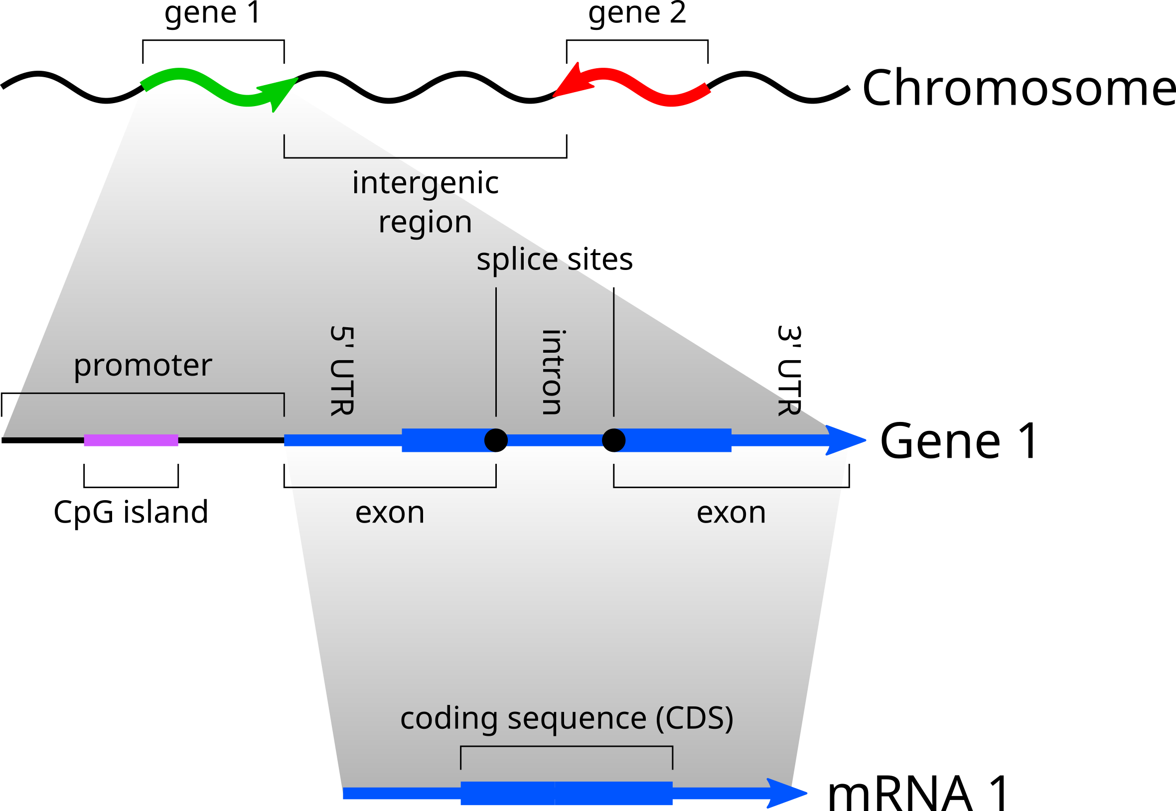
CpG islands are by definition regions of the genome rich in CG dinucleotides. Since they are enriched in CG dinucleotides, they have a higher proportion of Cs and Gs in their base composition. We can therefore model promoter sequence structure as switching between CpG islands rich in Cs and Gs, and non-CpG islands low in Cs and Gs. This is a discrete space, discrete time model, where the time dimension is the indices of the sites in the promoter, and a discrete random variable k specifies whether the present state is the start of the promoter (an empty sequence), CG-rich, or CG-poor.

Assume that from empirical observations of promoter sequences, we have inferred an HMM similar to the one below:

In this model, the first site of a promoter has an equal probability of a CG-rich or CG-poor state. This is because we begin at the start state with an empty sequence. The start state has equal transition probabilities 0.5 and 0.5 of transitioning to a CG-rich or CG-poor state at the next site respectively. There is no possibility of remaining in the start state at the next site, which is the zero probability above the circular arrow.

Conditional on a CG-rich state, for example if the first site is in a CG-rich state, the four nucleotides have the emission probabilities specified in the diagram. The probabilities of generating (or observing) A or T are 13% each, and the probabilities of C and G are 37% each. When in a CG-rich state, the transition probability to a CG-poor state is 37%, and complementary to this the probability of remaining in a CG-rich state is 63%.

The transition probabilities are symmetric for CG-rich and CG-poor, but the emission probabilities are not. If a site’s state is CG-poor, the probability of generating (or observing) A or T is 37% each, compared with 13% each for C or G. There is no probability on transitioning from the CG-rich or CG-poor states back to the start state, as that would make no sense.

We can simulate a promoter sequence based on this model using the following Python code:

import numpy

nucleotide_alphabet = "ACGT" # The alphabet of the nucleotide sites
state_alphabet = "SHL" # The alphabet of the states (start, CG High, CG Low)

# The emissions probability matrix. The rows correspond to the three states
# (start, CG-rich, CG-poor). The columns and the probability of emitting
# [A, C, G, T] conditional on the state.
emission_probs = numpy.array([
	[0.00, 0.00, 0.00, 0.00],
	[0.13, 0.37, 0.37, 0.13],
	[0.37, 0.13, 0.13, 0.37]
])

# The transition probabilities matrix. The rows correspond to the state at
# site i - 1, and the columns correspond to the probability of each state at
# site i
transition_probs = numpy.array([
	[0.00, 0.50, 0.50],
	[0.00, 0.63, 0.37],
	[0.00, 0.37, 0.63]
])

current_state = 0 # start at the start (state)
simulated_sites = "" # start with an empty sequence
simulated_states = "" # to record the sequence of states

# the length of promoter sequence to simulate
length = 100

for i in range(length):
	# choose a new state at site i, weighted by the transitional probability matrix
	current_state = numpy.random.choice(3, p = transition_probs[current_state])
	# choose a new nucleotide at site i, weighted by the emission probability matrix
	nucleotide = numpy.random.choice(4, p = emission_probs[current_state])

	# append the letter codes of the chosen state and nucleotide
	simulated_states += state_alphabet[current_state]
	simulated_sites += nucleotide_alphabet[nucleotide]

# print the simulation result
print(simulated_states)
print(simulated_sites)

This simulator uses a pseudo-random number generator (PRNG), and so will generate a different sequence each time it is run (unless we fix the “seed” of the PRNG). The following sequence of states and nucleotides was generated by running the simulator once:

HHHLHHHLLHLLHHHHLLLLHHHHLHLLLHLLHHHHHHHHHHLLHHHHHLHHHLHHHHLHLHHHHLHHLHHHLHHHHHHHLHHHHLHHHHLLLLHLHHLL
GCGGCCGATATACTACAGTTGGCTTGAATGAACCAGGCCCGGCGCGGACAACCTGGGCCCCGGCGGTCGCCCATACCGCAATGGGAGCCGTTAACTCGCT

Now let’s consider inferring splice site HMMs. The transcribed region of a gene, beginning at the transcription start site (TSS), is transcribed into RNA by the RNA polymerase II complex, and introns within the transcript are removed by the spliceosome complex or by self-catalysis. The 3’ end of the transcript is polyadenylated, meaning that a sequence of all As is added to the end of the RNA which was not derived from a complementary genomic DNA sequence.

The processed (spliced, polyadenylated, and otherwise covalently modified) RNA molecule is known as mRNA, and can be easily extracted by pulling out sequences with poly-A tails. Because transcription occurs simultaneously with splicing (splicing is also coupled with polyadenylation), extracted mRNA will already be spliced.

Given enough time and money for high coverage sequencing of mRNA, it is therefore possible to reconstruct the structure of all the genes in a genome. mRNA sequence reads can be aligned to a genome, and large gaps in alignment will correspond to introns used to predict gene structure. Alternatively, mRNA sequence reads can be assembled into a “transcriptome” of mRNA sequences, and those sequences can be aligned to the genome. Again the gaps in the alignment will correspond to introns. Inferring genes and gene structure in a genome is called “annotation”.

Using information in an existing annotation, we can infer an HMM for predicting genes and gene stucture. This will save much money and effort the next time we need to annotate a genome, as the annotation can be done entirely in silico rather than having to do more mRNA sequencing.

This time let’s consider a more realistic example. Here is a model of gene structure based on our knowledge that exons and introns are interleaved, so the 3’ site of an exon or intron is immediately followed by the 5’ site of an intron or exon respectively. The 3’ site cannot be followed by another 3’ site or a site interior to that exon or intron (otherwise it would be by definition not the 3’ site). The 5’ site also cannot be followed by another 5’ site for the same reason. While the model forces exons and introns to be at least 3 nucleotides in length, only one exon shorter than 3 nucleotides has ever been reported.

Note that we assume the sequence always starts somewhere inside an exon, and we are not modelling the transcription start site or polyadenylation, just splicing. Any “missing” arrows in the above model refer to transitions assumed to have zero probability.

Arabidopsis thaliana is a model plant with a well annotated genome. Using the latest genome assembly, TAIR10, and the GTF file of the latest genome annotation, we can extract the counts of nucleotide emission and state transition using the following script:

import csv
import numpy

# a function to read in the sequences from a FASTA formatted file, store the
# sequences in a dictionary structure, and return the dictionary
def read_fasta(fasta_path):
	fasta_file = open(fasta_path)
	l = fasta_file.readline()
	fasta_sequences = {}
	label = None
	sequence = None
	while l != "":
		if l[0] == ">":
			if label != None:
				fasta_sequences[label] = sequence

			label = l[1:].split()[0]
			sequence = ""
		else:
			sequence += l.strip()

		l = fasta_file.readline()

	fasta_file.close()

	if label != None:
		fasta_sequences[label] = sequence

	return fasta_sequences

# the order of columns in a GTF genome annotation file
gtf_columns = [
	"seqname",
	"source",
	"feature",
	"start",
	"end",
	"score",
	"strand",
	"frame",
	"attribute",
]

# only consider nuclear encoded genes, as mitochondrial and chloroplastic
# genes are more like bacterial genes and not expected to be predictable using
# the same model as nuclear genes
nuclear_chromosomes = {
	"Chr1",
	"Chr2",
	"Chr3",
	"Chr4",
	"Chr5",
}

# a function to read in a GTF genome annotation file, return which chromosome
# each gene comes from, and also return the half-open intervals of coding
# (CDS) sequences within the genome. The gaps between intervals correspond to
# introns.
def read_gtf(gtf_path):
	gtf_file = open(gtf_path)
	gtf_reader = csv.reader(gtf_file, dialect = csv.excel_tab)

	cds_regions = {}
	chromosome_map = {}
	for chromosome, source, feature, start, end, score, strand, frame, attribute in gtf_reader:
		transcript_id = attribute[attribute.find(" ") + 1:attribute.find(";")].strip('"')

		# make it easier for ourselves by only keeping positive strand exons
		if feature == "CDS" and strand == "+":
			if chromosome in nuclear_chromosomes:
				if transcript_id in cds_regions:
					cds_regions[transcript_id].append((int(start) - 1, int(end))) # convert to zero-based numbers with half-open intervals
				else:
					chromosome_map[transcript_id] = chromosome
					cds_regions[transcript_id] = [(int(start) - 1, int(end))] # convert to zero-based numbers with half-open intervals

	gtf_file.close()

	return cds_regions, chromosome_map

# read the latest Arabidopsis genome annotation file
araport11_cds_regions, araport11_chromosome_map = read_gtf("Araport11_GFF3_genes_transposons.201606.gtf")
araport11_order = sorted(araport11_cds_regions)

# read the latest Arabidopsis genome assembly file
tair10 = read_fasta("TAIR10_Chr.all.fasta")

# the order of letter codes of nucleotides, including ambiguity codes
alphabet = "ACGTWSMKRYBDHVN"

# for count matrix rows (and also columns for the transition matrix), the order is:
state_order = [
	"start",
	"exon interior",
	"exon 3'",
	"intron 5'",
	"intron interior",
	"intron 3'",
	"exon 5'"
]

emission_count_matrix = numpy.zeros([7, 15], dtype = "uint32")
transition_count_matrix = numpy.zeros([7, 7], dtype = "uint32")

# the number of transitions from the start state to the exon interior
# is equal to the number of transcripts
transition_count_matrix[0][1] = len(araport11_order)

# for each annotated transcript
for transcript_id in araport11_order:
	# get the sequence of the corresponding chromosome
	transcript_chromosome = araport11_chromosome_map[transcript_id]
	chromosome_sequence = tair10[transcript_chromosome]

	# get the CDS intervals
	cds_regions = araport11_cds_regions[transcript_id]
	n_exons = len(cds_regions)
	n_introns = n_exons - 1

	# the number of exon/intron transitions is equal to the number of introns
	transition_count_matrix[1][2] += n_introns
	transition_count_matrix[2][3] += n_introns
	transition_count_matrix[3][4] += n_introns
	transition_count_matrix[4][5] += n_introns
	transition_count_matrix[5][6] += n_introns
	transition_count_matrix[6][1] += n_introns

	for i, interval in enumerate(cds_regions):
		cds_start, cds_end = interval

		transition_count_matrix[1][1] += (cds_end - cds_start) - 2 # add all the interior sites of the exon

		# store interior nucleotides in count matrices
		for j in range(cds_start + 1, cds_end - 1):
			interior_exon_nucleotide = alphabet.index(chromosome_sequence[j])
			emission_count_matrix[1][interior_exon_nucleotide] += 1

		five_prime_exon_nucleotide = alphabet.index(chromosome_sequence[cds_start])
		three_prime_exon_nucleotide = alphabet.index(chromosome_sequence[cds_end - 1])

		if i == 0: # if the first exon, 5' nucleotide will be adjacent to the 5' UTR and not to a splice site
			emission_count_matrix[1][five_prime_exon_nucleotide] += 1
		else: # otherwise it is adjacent to a splice site
			emission_count_matrix[6][five_prime_exon_nucleotide] += 1

		if i == n_exons - 1: # if the last exon, 3' nucleotide will be adjacent to the 3' UTR and not to a splice site
			emission_count_matrix[1][three_prime_exon_nucleotide] += 1
		else: # otherwise it is adjacent to a splice site
			emission_count_matrix[2][three_prime_exon_nucleotide] += 1

			# if not the last exon, count nucleotides in the intron that follows
			intron_start = cds_end
			intron_end = cds_regions[i + 1][0]

			transition_count_matrix[4][4] += (intron_end - intron_start) - 2 # add all the interior sites of the intron

			# store interior nucleotides in count matrices
			for j in range(intron_start + 1, intron_end - 1):
				interior_intron_nucleotide = alphabet.index(chromosome_sequence[j])
				emission_count_matrix[4][interior_intron_nucleotide] += 1 # non-splice-site intron nucleotide

			five_prime_intron_nucleotide = alphabet.index(chromosome_sequence[intron_start])
			three_prime_intron_nucleotide = alphabet.index(chromosome_sequence[intron_end - 1])

			emission_count_matrix[3][five_prime_intron_nucleotide] += 1 # the 3' ends of exons are always splice sites
			emission_count_matrix[5][three_prime_intron_nucleotide] += 1 # the 5' ends of exons are always splice sites

transition_matrix_path = "transition_matrix.csv"
emission_matrix_path = "emission_matrix.csv"

transition_matrix_file = open(transition_matrix_path, "w")
emission_matrix_file = open(emission_matrix_path, "w")

transition_matrix_writer = csv.writer(transition_matrix_file)
emission_matrix_writer = csv.writer(emission_matrix_file)

transition_matrix_writer.writerow(state_order)
emission_matrix_writer.writerow(alphabet)

for t_row_i, transition_row in enumerate(transition_count_matrix):
	# avoid dividing by zero when no transitions are out of this state
	transition_probabilities = transition_row / max(numpy.sum(transition_row), 1)
	transition_matrix_writer.writerow(transition_probabilities)

for e_row_i, emission_row in enumerate(emission_count_matrix):
	# avoid dividing by zero when no emissions are observed for this state
	emission_probabilities = emission_row / max(numpy.sum(emission_row), 1)
	emission_matrix_writer.writerow(emission_probabilities)

transition_matrix_file.close()
emission_matrix_file.close()

Based on the emission and transition counts, we can fill in the probabilities of our splice site HMM:

Any arrows in the above diagram without explicit probabilities are where we assume that transition occurs with 100% probability. Here are some notable things that can be observed from these empirical probabilities:

• The 5’ and 3’ nucleotides of introns are almost invariably G
• The 5’ and 3’ nucleotides of exons are G most but not all of the time
• The rate of transition from exon to intron is lower than intron to exon, which implies that exons will be longer than introns
• Introns are enriched in T, an phenomenon reported by Ko et al. in 1998.

For more on Hidden Markov Models, see Chapter 3 of Biological sequence analysis by Durbin et al.

Update 13 October 2019: for another perspective on hidden Markov models, consult Chapter 10 of Bioinformatics Algorithms (2nd or 3rd Edition) by Compeau and Pevzner.